RDP 8808: Consumption and Permanent Income: The Australian Case 2. Testable Implications of the Life Cycle Model
October 1988
- Download the Paper 865KB
The life cycle model of consumer behaviour can be tested by examining either consumption or savings behaviour. The most popular approach has concentrated on the consumption side – and this paper will follow that path.[2]
Consider a representative consumer who is faced with a choice of consumption in each period given an initial asset stock and an uncertain income stream. Assume that the only uncertainty is the future stream of income.
The consumer's problem can be written:


| where | δ | = | rate of time preference |
| Ct | = | real consumption in period t | |
| At | = | real non-human wealth at start of period t | |
| Yt | = | real after-tax labour income in period t | |
| rt | = | real after-tax interest rate in period t | |
| and | Et | = | denotes expectation at time t |
| U(Ct) | = | denotes the utility derived from consumption in period t |
Solving this problem and assuming a bounded solution gives:


Equation (3) gives the familiar result that the consumer equates the marginal utility from consumption across time, adjusted for the rate of time preference and the real return from postponing consumption.
The difference equation (4) can be solved to find:

where

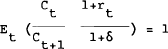
Equation (5) can be rewritten:


Ht can be interpreted as the expected real value of human wealth at start of period t. It is the present discounted value of the expected future stream of after-tax labour income where the rate used to discount the stream of income is the real return to holding financial wealth.
Equation (7) shows that the present value of consumption expenditure should equal the initial assets plus human wealth. This states that the optimal solution for consumption is to consume all resources during the consumption horizon.
The time path of consumption depends on the form of the utility function. As an illustration, assume that utility is a log function of the level of consumption:

We can rewrite (3)
Based on Hansen and Singleton (1983), it can be shown that by assuming C and r are jointly log normally distributed, we can make some convenient simplifications. If we let

and assume Xt = log xt
where X ~ N(µ, σ2)
we have E(xt+1|It) = exp (µ + σ2/2)
or log E(xt+1|It) = µ + σ2/2
and E(Xt+1|It) = E(log Xt+1|It) = µ
Therefore, log E(xt+1|It) = E(log Xt+1|It) + σ2/2
Using this transformation plus the assumption of rational expectations, it can be shown that (10) holds.

where 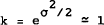 since σ ≃ .01
k can be interpreted as a linearization error which we will ignore.
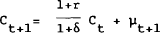
µt+1 is white noise. It can be seen from (10) that if r is constant and equal to δ, then consumption is a random walk.
Combining (10) and (7) and ignoring k, it can be shown that:

Where et is a white noise disturbance. For steady state consumption to be constant we require that δ=r. Substituting this into (11) gives a steady state relation

Equation (12) implies that consumption in each period is the annuity value of human plus non-human wealth. This can also be defined as permanent income (see Flavin (1981)). Note that this result differs slightly from Flavin's because of the discrete approximation for the budget constraint we use in (4) which is the standard approach. If it is assumed that At+1 = (1+rt) At + Yt – Ct then we find the result in Flavin.
Generally, it is convenient to express (11) as:

where α will not necessarily be independent of r, for example if bequests are important, and depending on the form of the underlying utility function.
To estimate the permanent income model it is possible to follow a variety of approaches, based on the different stages of substitution in the equations above. Before proceeding, it is convenient to introduce a generalisation to the above model. Assume that there are two types of agents in the economy. Agents of type x consume out of permanent income (YP) and agents of type v consume out of current (or disposable) income (Y). We assume that agents of type x receive a fixed share Ω of total income and type v agents receive (1−Ω) of total income.[3] Then:

assuming that all assets are held by type X agents.
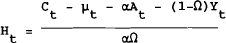
The model for aggregate consumption becomes:

In principle, (14) can be estimated given data for C,A,H and Y. Unfortunately, data on human wealth is not available. One alternative is to approximate the value of future income by a distributed lag on past values of income. The problem with this as pointed out by Lucas (1976) is that expectations are inadequately represented.
(a) The Hall Approach
Other alternatives exploit the implications of assuming rational expectations. One such alternative is to estimate the Euler equation (3) directly following Hall (1978). This requires an assumption of the form of the utility function. Again, by assuming log utility, a constant r and rational expectation we have:
or

where Et (µt+1) = 0
Note that if γ=1 (i.e., δ=r) then consumption follows a random walk. Again, introduce two types of agents.


Aggregate consumption becomes:

or

Note that if r=δ, then γ=1 and  is a random walk. The
change in aggregate consumption is then only a function of the change in income.
is a random walk. The
change in aggregate consumption is then only a function of the change in income.
Equation (19) can be used to test the joint hypothesis of permanent income, rational expectations and that a share of consumption is determined by current income, though there are some econometric problems to overcome. The first problem we need to consider is the time series properties of C and Y. If C and Y are non-stationary, then as shown by Mankiw and Shapiro (1985), we may encounter bias in testing for the significance of γ, especially if we have a stationary series as a dependent variable and non-stationary series as independent variables. Stock and West (1987) show that the bias from this problem is avoided if the equation can be re-written with only trend stationary variables as dependent variables. The standard t-tests will then be asymptotically valid. In our model, if C and Y are cointegrated,[4] we can, in fact, rewrite the model with only trend stationary variables on the right hand side. For example, equation (19) can be rewritten:

Under the null hypothesis, γ=1, Ω=1 and therefore C has a unit root. If Y also has a unit root and C and Y are cointegrated with a cointegrating factor of (1−Ω) then ΔY and (C – (1−Ω)Y) will both be stationary. A problem emerges if γ>1 and if C and Y are not cointegrated. However, C and Y can be tested for cointegration before carrying out the analysis and the residuals from this equation can be tested for non-stationarity which could be an alternative test for cointegration if γ ≠ 1.
Further problems occur because ΔYt will likely be correlated with µt and, therefore, needs to be instrumented out. This may be a problem if Yt is also a random walk, since by definition there are no instruments for ΔYt. This also causes problems since from (19), if ΔY is white noise then the hypothesis that consumption is driven by current income is indistinguishable from the permanent income hypothesis; current income is the best guess of permanent income.
(b) The Hayashi Approach
An alternative approach follows Hayashi (1982). The essence of Hayashi's approach is to use the equation for the evolution of human wealth implied by equation (8) to substitute out for human wealth. Hayashi also introduces the possibility that the rate used to discount future income streams is different to the return on financial assets, possibly due to capital market imperfections.
Assuming rational expectations, equation (8) can be rewritten :


that is, εt is the revision to expectations over the path of Yt, with EtYt+s defined as the expectation at time t of Yt+s. rh is the rate used to discount future income which we now allow to differ from r. For convenience assume rh is constant.
Using (14), we have
which can be substituted into (20) to find
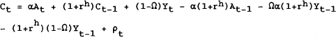

Hayashi proceeded to estimate (21) and (14). Recent work has shown that this is problematic if C and Y are non-stationary series. Therefore, the equations are estimated in differenced form here.


Note that by assuming rh=r=δ we can manipulate equations (22) and (23) to find:

which is our test for the Hall model assuming γ=1 (i.e., r=δ). This is not surprising since the two approaches are only rearrangements of the same set of first-order condition and budget constraints. The advantage of the Hayashi approach is that it allows us to explore the assumptions about the rates of return used to calculate human wealth and financial wealth.
We make different assumptions about the relationship between r (the real return on financial assets) and rh (the real rate used to discount future income). Firstly, if we assume both are constant and equal we can estimate (22) and (23) together to find estimates for α, Ω and the constant rh. These results can be used to test the permanent income hypothesis given data on financial wealth. If the permanent income hypothesis alone explains consumption, then the estimate for Ω will be close to unity. On the other hand, if consumption can be explained purely by current income, then Ω will be close to zero, and the other parameters will be insignificant.
There are some econometric problems with directly estimating equations (22) and (23). The issue of non-stationarity has already been dealt with. Other econometric problems emerge because we have by construction:

and

Also note that At is not in the information set It−1 on which the expectation of εt is conditioned. Therefore E(εt At) ≠ 0. We need a set of instruments that are uncorrelated with µt and µt−1. The NLIV (non-linear instrumental variable) technique suggested by Hayashi is used here.
A third test for the relevance of the permanent income hypothesis was suggested by Flavin (1981). Flavin concentrates on the effect of innovations in income on innovations in consumption. She explicitly models the time series of consumption and income as a bivariate autoregressive process imposing cross equation restrictions from the rational expectation assumption. This has been criticised by Mankiw and Shapiro (1985) amongst others because of the inappropriate test statistics when consumption and income follow random walks. In this case, the test of excess volatility of consumption will be biased. Engle and Granger (1987) further point out that if C and Y are cointegrated then a technique such as Flavin's will be misspecified.[5] We do not pursue the Flavin approach further.
Footnotes
However, see Campbell (1988) and Deaton (1986) for an alternative approach based on savings behaviour. [2]
In terms of a classical framework, this dichotomy might be interpreted as assuming that one group (call them workers) consume all their current income, do not save (except via government pensions etc.) and thus do not receive property income, while the other class (call them capitalists) consume their permanent income, accumulating savings in the process. The stability conditions of the two class system could be derived, as in Pasinetti (1962), and would probably depend upon the savings rate of the capitalist class being above some crucial value. [3]
Two series (C,Y) will be cointegrated if they are the same order of integration and if the residuals from the regression Ct=α+βYt+εt, are stationary. [4]
See Macdonald and Kearney (1987) for estimates of a permanent income model using cointegration techniques. [5]