RDP 9307: Explaining Forward Discount Bias: Is it Anchoring? 5. Empirical Results

5.1 Calibrating the Model

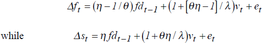
We derive empirical results for the special case of the model and hence the exchange rate evolves according to equation (11).^[20] We require values for five parameters: θ, λ, σ_m, σ_e and β. Estimates for the first four come from real-world data. 1/θ is the rate at which goods-prices and the interest differential adjust to money supply shocks and is estimated from the time-series properties of 3-month interest differentials between pairs of the countries US, UK, (West) Germany and Japan. Details of the interest rates used are in the Data Appendix. The AR(1) equation describing the evolution of (i – i^*)_t (equation (6)) is estimated by OLS leading to the estimates for θ shown in Table 1 (p 36).^[21] To cover the range of results in Table 1, we generate numerical results with θ = 6 periods and θ = 50 periods.^[22]

Estimates of the semi-elasticity of money demand with respect to the interest rate, λ, are derived from money demand functions estimated for the G-7 by Fair (1987). Details are presented in Appendix D and the resulting parameter values are shown in Table 2. When θ = 6 periods (50 periods), the derived value of λ implies that a 1% increase in the nominal money supply leads to contemporaneous fall in the domestic interest rate of 2.0% p.a. (0.7% p.a.).

The standard deviation of nominal money shocks, σ_m, is set so that the standard deviation of the interest differential, σ(i–i^*), equals 1.9% p.a. (the standard deviation of the Japan – Germany interest differential from Table 1, chosen because these two countries had comparable inflation rates over the 1980s). The AR(1) specification for (i–i^*)_t implies that , which allows σ_m to be determined for given θ and λ. Again, the results are shown in Table 2.

The standard deviation of long-run real exchange rate shocks, σ_e, is set so that the model generates an appropriate amount of exchange rate volatility. Baille and Bollerslev (1989) examine the stochastic properties of the nominal exchange rates of France, Italy, Japan, Switzerland, UK and (West) Germany against the US dollar, 1980–85. For 4-week periods, these exchange rates are well modelled by the process

where b_j and σ_Δsj are country-specific constants and σ_Δsj ranges from 0.029 to 0.037 with a mean over the six exchange rates of 0.034. Choosing σ_e = 0.031 for the model ensures that model values of σ_Δs always fall within the range found by Baille and Bollerslev.^[23]

We present results for two values of β. With the goods market in long-run equilibrium (p_t = _t), the impact response to a money shock ν_t+1 is Δs_t+1 = 0 with only anchored traders in the market and Δs_t+1 = ν_t+1(1+θ/λ) with only rational traders. We use values for β derived from the market's impact response to this shock when managed wealth is divided equally between the traders. When α = 1/2, if the spot exchange rate immediately jumps halfway to the value it would take were the market fully rational (Δs_t+1 = ν_t+1(1+θ/λ)/2), then from equation (11),

and we describe the anchored traders as ‘weakly anchored’. Alternatively, when α = 1/2, if the spot exchange rate immediately jumps only one-tenth of the way to the value it would take were the market fully rational, Δs_t+1 = ν_t+1(1 + θ/λ)/10, then

and we describe the anchored traders as ‘strongly anchored’.

5.2 Endogenous Determination of the Proportion of Anchored Traders

With a proportion α of market wealth managed by anchored traders, define R^k (α,n) as the gross real return trader k earns over n periods on the portfolio she manages. Further, define Z(α,n) ≡ R^α(α,n) – R^r (α,n) as the excess real return earned by anchored traders over n periods. Then, as demonstrated in Appendix E,

where .

For given α, we use (15) to derive estimates of p(α,n) ≡ Pr[Z(α,n) > 0], the probability that the anchored traders' chosen portfolio outperforms the rational traders' portfolio over the assumed horizon of investors, n. From these estimates, we also derive estimates of the proportion of anchored traders in the market in the long-run. We assume that investors follow a simple decision rule. Every n periods, they compare the relative performance of the two types of traders over the past n periods. When type-k traders (k = a or r) had the better performance, investors increase the proportion of wealth entrusted to them by a constant q, subject to the constraint that the share of market wealth entrusted to either type of trader never falls below zero.^[24] Then the evolution of α follows a Markov chain

where the subscript T refers to successive n-period time-intervals.^[25]

We can now derive the long-run stationary probability distribution of α. We assume α₀ = 0 and q ∈ {0.1,0.3,0.5,1.0}. Then there are at most eleven states for the Markov chain, αⁱ = i/10, i = 0,..., 10, and at all times, α_T must take one of the values αⁱ. The stationary probability distribution for α is defined by the probabilities pⁱ

From this probability distribution, we derive the long-run average proportion of anchored traders in the foreign exchange market, , given by

and the long-run average coefficient on the forward discount in equation (11), ,

5.3 Results and Discussion

Figure 3 shows empirical estimates of p(α,n) for one set of parameter values (θ = 6 periods; strongly anchored traders) and for three assumed horizons for investors (one, three and ten years).^[26] Table 3 reports long-run averages of the proportion of anchored traders in the market, , and the coefficient on the forward discount in the standard test of forward discount bias, , derived for different assumed values of the Markov chain parameter, q, in equation (16).

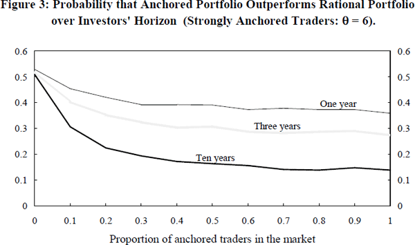
For all sets of parameter values, p(0,n) ≈ 0.5 and p(α,n) falls monotonically as α increases.^[27] But it is noteworthy that even over long horizons, the chance that the anchored traders' portfolio outperforms the rational traders portfolio is not so small. An example makes the point. With θ = 6 and market wealth divided equally between rational and strongly anchored traders, η takes the value η ≈ −0.9. Thus, the forward discount is a very significantly biased estimate of the future exchange rate change. Despite this, over a three year (ten year) horizon, the portfolio chosen by the anchored traders (who use the forward discount as the anchor for their expectations of the exchange rate change) gives a higher return than the rational portfolio 31% (16%) of the time. This example highlights the general point that unpredictable exchange rate movements are so big that only a small advantage is imparted to those (rational) traders who understand the true relationship between interest rates and the exchange rate.

The results in Table 3 imply, over a wide range of parameter values, that a significant proportion of anchored traders survive in the long-run and that they induce substantial bias in the forward discount. The largest value of in the Table is = 0.63 while for strongly anchored traders and shorter investor horizons, the value of is close to zero or negative. As reported in Section 2, the empirically estimated coefficient on the forward discount in the corresponding regression (equation (1)) is often negative. For the range of parameter values investigated, while the model does not often generate negative values of , it always generates strong forward discount bias in the direction consistently observed empirically.

While one might quibble with the specification chosen for the anchored traders' expectations, a strong message emerges from these empirical results. If rational agents in the foreign exchange market are risk-averse or liquidity-constrained, the rational expectations solution for the exchange rate (allowing for risk-aversion) is a fragile one. Unpredictable exchange rate movements are so big that there are no strong grounds for presuming that agents with quite different expectations will be driven from the market. This may help explain why economists have had such difficulty modelling the short-run behaviour of exchange rates.

5.4 Comparison with Other Work

We begin this sub-section by showing that the model generates several of the empirical regularities described in the literature. McCallum (1992) presents a useful summary of these regularities with eight OLS regressions using over twelve years of monthly data for $/DM, $/£ and $/¥ exchange rates. For the first seven regressions, Table 4 compares his $/DM results (which are representative) with results derived from a simulation of the model. The first regression in the table is the standard test for forward discount bias and, while the model produces a negative coefficient on the forward discount, it is significantly less negative than McCallum's coefficient. As discussed earlier, for the range of parameter values investigated, the model does not generate large negative values of this coefficient ().

We now explain the model results for the remaining regressions in the table. The model results for regressions (2) and (3) are a consequence of the fact that s and f are co-integrated I(1) variables with co-integrating vector, s_t = f_t. This explains both the estimated slope coefficient and the very high regression R². Further, in the model,

Since e_t is much larger than all the other terms on the right-hand-side of either of these equations, a regression of Δs_t on Δf_t is rather like regressing e_t on itself, which explains the model results for regression (4). Lagging the right-hand-side variable in regression (4) generates regression (5), and the relationship disappears because, for the model, (5) is rather like regressing e_t on e_t–1. Similar logic explains the model results for regressions (6) and (7). Regression (6) is like regressing e_t + e_t–1 on e_t–1; which explains both the slope coefficient and the fact that R² ≈ 1/2. Regression (7) is like regressing e_t + e_t–1 + e_t–2 on e_t–1 + e_t–2; which again explains the slope coefficient and the fact that R² ≈ 2/3. As is clear from the table, there is a very close fit between the model results and all the empirical results reported by McCallum.

The last OLS regression reported by McCallum is

For each of his three exchange rate datasets, he shows that a₁ ≈ 1 – a₂ ≈ b, where b is the coefficient on the forward discount in the standard test for forward discount bias (regression (1) in Table 4). Equations (3) and (13) imply for the model that

where c₁ ≡ 1 – c₂ ≡ η, and η is the model coefficient on the forward discount in the standard test for forward discount bias (equation (13)). Thus, again, McCallum's empirical results are reproduced by the model.

We conclude this sub-section with a potentially serious shortcoming of our assumed money supply process. We assume the log-level of the money supply follows an ARIMA(0,1,0) process while Lyons (1990) points out that quarterly log-changes in the US money supply are approximately ARIMA(0,1,1). Lyons' observation implies that a current shock to the money stock leads rational agents to adjust their estimates of future money growth. So a money shock has both a direct effect on the exchange rate as well as an indirect growth-rate effect. Our assumed money supply process ignores the indirect growth-rate effect because it assumes that shocks to the money stock are independent of each other.

There are two relevant comments. Firstly, for realistic parameter values, the importance of the indirect growth-rate effect is unclear. If money supply growth rate innovations are truly permanent, the indirect effect is about twice as large as the direct effect (Lyons' Table 5). But if they are long-lived but temporary, as seems more plausible, his Table 3 suggests that the indirect effect is much less important. Secondly, recall our observation that only a small advantage is imparted to those (rational) agents who understand the true relationship between interest rates and the exchange rate. This key observation explains the long-run survival of a significant proportion of anchored traders. While Lyons' evidence represents a potential challenge to this observation, other empirical evidence (footnote 4) is strongly supportive of it. Note in particular the Meese and Rogoff (1983) finding that knowledge of the actual future money supply hardly helps at all to explain the level of the future exchange rate for horizons up to a year. To summarise, Lyons' point is an important conceptual one, but the balance of evidence strongly suggests that it does not overturn the key assumption on which our results depend – that only a small advantage is imparted to those who understand the true relationship between interest rates and the exchange rate.

Footnotes

As will soon be clear, the size of the unpredictable real exchange rate shocks, σ_e, determines our empirical results. But these shocks are the same in both cases of the model, so results for the general case should be very similar to those reported below. However, deriving results for the general case requires specifying values for two more parameters (γ and κ). [20]

A constant is included in the OLS regression to allow for different inflation rates between countries. Augmented Dickey-Fuller tests (Appendix D) imply, at least for the Japan–Germany and Japan–US interest differentials, that the hypothesis of a unit root can be rejected with some confidence. An alternative method for estimating θ using the autocovariance of the interest differentials gives similar results. [21]

θ = 50 periods is chosen because the OLS estimates of θ are biased downward. θ = 6 (θ = 50) implies that the half-life for goods-price adjustment is 3.5 months (32 months) which probably spans the plausible range for goods-price stickiness. [22]

Exchange rate volatility in the model is dominated by real exchange rate shocks, but it also depends weakly on nominal shocks. Equations (11) or (13) imply that:
. With σ_e = 0.031 and θ = 6 (θ = 50), σ_Δs ranges from 0.031 (0.031) when α = 1 to 0.033 (0.037) when α = 0. [23]

We assume that both types of traders always have at least an infinitesimal market presence so that investors can always observe their relative performance. One way to motivate this assumption is to imagine that new anchored and rational traders enter the market every period, but only when they are successful do they attract a non-negligible fraction of market wealth. [24]

Incorporating this Markov chain for α_T into the rational traders expectations in Section 4 would add little of substance but greatly complicate the algebra. Our decision rule for investors is similar to the ‘Imitation Based on Realised Returns’ rule of De Long et. al. (1990a). As an alternative, the investors' decision rule could be based on the traders' relative realised utilities rather than their realised returns. This alternative assumption would reduce the proportion of anchored traders in equilibrium but would not change the qualitative nature of our results. De Long et. al. present reasons for preferring a decision rule based on realised returns: ‘we find it plausible that many investors attribute the higher return of an investment strategy to the market timing skills of its practitioners and not to its greater risk. This consideration may be particularly important when we ask whether individuals change their own investment strategies that have just earned them a high return. When people imitate investment strategies, they appear to focus on standard metrics such as returns relative to market averages and do not correct for ex ante risk’ (p. 724). Shiller (1992) presents supporting evidence (p. 70–74). [25]

Each year contains thirteen 4-week periods, and for each (α, n) pair, 10,000 realisations of the random variable Z(α,n) are used to generate results. [26]

Despite the fact that E Z(0,n) = 0, in all cases p(0,n) > 0.5 because the random variable Z(0,n) is slightly skew when n > 1. [27]