RDP 9610: Share Prices and Investment 3. Share-Market Efficiency
December 1996
- Download the Paper 121KB
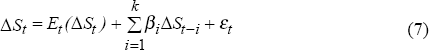
The Efficient Market Hypothesis states that the share market is weak-form efficient if share prices incorporate all historical information such that investors are unable to predict future share-price movements from previous movements.[7] The implication of this definition is that share-price returns should be uncorrelated with historical returns. One method for testing share-market efficiency involves testing whether share-price returns (ΔSt) are correlated with past returns, that is testing the significance of the βi's in Equation (7). One problem with this methodology is that it assumes that the model of expected returns (Et (ΔSt)) is reliable. As such, these tests are actually joint tests of share-price efficiency and whether the model of expected returns is correctly specified (Fama 1991).
where: εt ~ iid(0,σ2)
In the earlier literature, expected returns were assumed to be constant, and so efficiency tests were simply tests of whether share price returns (ΔSt) were correlated with past returns (Fama 1970). These tests often found that share-price returns were predictable from past returns, that is inefficient.
The view that expected share-price returns are invariant over time is now generally acknowledged as being too simplistic. In the more recent literature, Fama (1991) and others[8] argue that rather than indicating inefficiencies, predictability of long-run returns could indicate that expected returns are themselves serially correlated over time. That is, expected returns are time-varying. For example, if an asset's expected return is equal to the risk-free rate plus a constant instrument-specific risk premium, the expected return is likely to be serially correlated if the risk-free rate is related to the business cycle (Fama and French 1989).
Simple versions of this proposal test whether share-price returns in excess of the risk-free rate are correlated over time. Overseas studies tend to find that the results are largely dependent on the frequency of the data used.[9] They find that ‘excess’ returns are autocorrelated over short horizons but that this correlation dissipates over longer horizons.
More complicated versions of the ‘time-varying’ literature explicitly model expected returns with respect to both long and short-run factors. These models test whether short-run movements in share prices are anchored to a long-run fundamental share price. For example, Tease (1993) models expected returns to reflect the present value of expected nominal income flows and shows that although speculative factors may drive returns away from their equilibrium in the short run, returns gradually revert to their fundamental value.
These models appear to indicate that share prices deviate from their fundamental value and are, therefore, inefficient. Recent literature suggests, however, that even rational investors who typically sell high and buy low (and therefore stabilise prices) may rationally and profitably destabilise prices in the short run.[10] For example, technical traders may sell into a declining market if they believe that a price movement is likely to continue, possibly as a result of investors who ‘trend chase’ or who trade on the basis of stop-loss or portfolio insurance strategies. With this literature in mind, these tests of efficiency which establish short-run share-price deviations from fundamentals should be broadly interpreted as tests establishing long-run efficiency and short-run speculative dynamics.
3.1 Tests of Share Market Efficiency
There are few tests on weak-form efficiency in Australian share prices. Groenewold and Kang (1993) tested both weak and semi-strong form efficiency using monthly data in the Australian share market between 1980 and 1988 and found no evidence of share-market inefficiency. Blundell-Wignall and Bullock (1992) found share prices to be inefficient over short time horizons but that they reverted to their fundamental value in the long run.
In this section we test for Australian share-market efficiency under the alternative assumptions of constant and time-varying expected returns. Although it is not possible to fully resolve the question of share-market efficiency due to the problem of unobservable expected returns, our results reach similar conclusions – that there is evidence of share-price inefficiency over short horizons but little evidence of share-price inefficiency over longer horizons.
3.1.1 Tests for autocorrelation
Our tests of return predictability follow the literature by estimating autocorrelation coefficients and testing their significance with the Ljung-Box Q test. We test for efficiency under the alternative assumptions of constant and time-varying expected share-price returns.[11] The null hypothesis is that the share market is efficient. That is, that the first k autocorrelations are not significantly different from zero.
The results under the alternative assumptions of constant and time-varying expected share-price returns are very similar (Table 1). We find that over shorter horizons (daily, monthly and quarterly) positive serial correlation is present, while over a long horizon (annual), it is less evident.[12] These results are in line with overseas studies (Poterba and Summers 1988; Tease 1993).
| Ljung-Box Q Statistics | ||
|---|---|---|
| Constant expected return | Time-varying expected return | |
| Daily | 254.4 ** | 254.6 ** |
| 1987–1996 | (0.00) | (0.00) |
| Monthly | 111.7 ** | 113.5 ** |
| 1959–1996 | (0.00) | (0.00) |
| Quarterly | 36.0 ** | 48.8 ** |
| 1936–1996 | (0.00) | (0.00) |
| Annual | 8.6 * | 10.3 * |
| 1889–1995 | (0.03) | (0.02) |
|
Notes: * and ** denote significance at the 5% and 1% level, respectively. The marginal significance levels (p-values) are in parentheses. The number of autocorrelations (k) tested are 3 for annual data, 12 for quarterly data, 36 for monthly data and 100 for daily data. |
||
Figure 1 which plots the correlation coefficients shows that the incidence of positive and significant coefficients declines as the frequency of the data declines. Tentatively, this can be interpreted as providing some evidence that even though share prices are inefficient in the short run, they revert to their fundamental value over time.
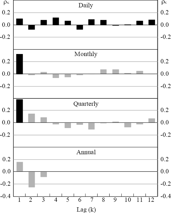
Note: The black bars indicate that the autocorrelation coefficient is significantly different from zero at the 1% level of significance.
One problem with this approach is that the sample period covers quite diverse stages in the development of the Australian share market. Similar correlation tests were made on rolling 36-month periods from 1962. The results are presented in Figure 2 which shows that the Ljung-Box Q statistics tend to be smaller (and less significant) in the eighties and nineties than in the previous two decades. This would seem to indicate that the Australian share market has become more efficient over time and could explain why some papers find evidence of inefficiency while others have failed to do so.

Note: Shaded area indicates acceptance of the null hypothesis of no serial autocorrelation at the 5% level of significance.
Another criticism of this simple approach is that the All Ordinaries Share Price Index incorporates the prices of infrequently traded shares. The implication of this is that while macroeconomic developments such as exchange rate movements or changes in the company tax rate will be immediately reflected in the prices of the frequently traded shares, it may take some time to be reflected in the prices of the less frequently traded shares. Conceptually, the lagged response of the infrequently traded share prices to new information may be spuriously interpreted as indicating autocorrelation. In an attempt to determine whether there is any inherent bias caused by infrequently traded shares, the same autocorrelation tests were re-estimated using the ‘narrower’ 50-Leaders Share Price Index. While the 50-Leaders Index is only available from 1980, no qualitative difference was evident in the results.
3.1.2 Modelling expected share price returns
A more formal method of testing for efficiency assuming time-varying expected returns is to use an unrestricted error correction model of the form specified in Equation (8). It is assumed that, in the long run, share prices reflect the present value of expected future cash flows. This is estimated using the log of real corporate profits after interest together with the general price level.[13] To model the short-run dynamics, the log differences of nominal share prices, real corporate profits after interest, the general price level (inflation) and oil prices are included with four lags.[14] The cost of capital, proxied by the 10-year bond yield, is also included with four lags. The null hypothesis tested here is that if share prices are characterised by speculative dynamics in the short run, and a return to equilibrium over time, then the lagged response to changes in share prices (ν) should have a positive and significant coefficient and there should be evidence of cointegration in the long run (that is, γ should be negative and significant).
As a preliminary to estimation, unit root tests were conducted and the results are presented in Appendix A. The tests showed that all the variables in Equation (8) are integrated of order one. We chose to consider the cost of capital series (estimated by the nominal bond yield) as stationary notwithstanding the unit root test result since the series is necessarily bounded.
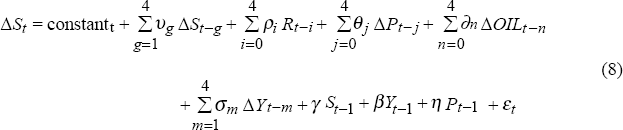
| where: | S = nominal share prices |
| R = cost of capital (10-year bond yield) | |
| P = general price level | |
| OIL = oil price | |
| Y = real cash flow |
The results are presented in Table 2. Of the short-run explanatory variables, the coefficients for the change in real cash flows and inflation were insignificant and were subsequently dropped to arrive at our preferred equation. The change in share prices and the cost of capital (each with four lags) are significant and have the expected sign. Real cash flows and the general price level are significant in the long run. The change in oil prices, although insignificant, were retained to control for supply-side shocks. Our preferred equation satisfies the diagnostic tests for serial correlation, normality and autoregressive conditional heteroscedasticity.
| Quarterly 1962:Q1–1996:Q1 (8) |
|
|---|---|
| Explanatory variables – short run: | |
| constant | −0.01 (0.0) |
| ΣΔSt–k | 0.37** (21.4) |
| ΣRt–k | −0.43** (30.6) |
| ΣΔOilt–k | −0.15 (9.3) |
| Explanatory variables – long run: | |
| γ (Cointegration test) |
−0.10** (2.6) |
| Yt–1 | 1.02* (2.1) |
| Pt–1 | 0.71** (2.6) |
| Summary statistics: | |
 |
0.23 |
 |
0.08 |
| Serial correlation test (χ2(4)) | 0.24 |
| Normality test (χ2(2)) | 0.09 |
| ARCH Test (χ2(1)) | 0.46 |
Notes: * and ** indicate the coefficients are significantly different
from zero at the 5% and 1% significance levels. For the short-run explanatory
variables the figures in parentheses are chi-squared statistics testing the null
hypothesis that the coefficients are jointly equal to zero. For the long-run
explanatory variables, the Bewley (1979) transformation was applied to obtain
interpretable t-statistics (shown in parentheses). The cointegration test proposed
by Kremers, Ericsson and Dolado (1992) was employed. ‘ |
|
In line with previous studies (Blundell-Wignall et al. 1992; Tease 1993), these results support the hypothesis of short-run speculative dynamics – the coefficients on the lagged changes in share prices are positive and jointly significant at the one per cent significance level. There is also evidence of cointegration, suggesting that share prices return to their fundamental value in the long run.
In summary, while there is evidence that share prices are inefficient over shorter time horizons these results appear to be biased somewhat by the earlier years in the Australian share market when the capital markets may have been less liquid. Reflecting the changes in Australian financial markets in the eighties, there is evidence that the liquidity in the market has improved and share price inefficiencies have been reduced.
Footnotes
In the early efficiency literature (summarised in Fama (1970)), efficiency is classified into three testable forms – weak, semi-strong and strong. In Fama (1991) these definitions are refined into three equivalent categories; return predictability tests which include all models that forecast returns using historical share prices, dividends and earnings yields; event study tests which are concerned with whether share prices efficiently adjust to new, publicly available information; and private information tests which examine whether insiders have information which is not fully reflected in share prices. As such, return predictability tests of efficiency under the Efficient Market Hypothesis (weak-form tests) is the least stringent definition of efficiency but is the most relevant definition from a macroeconomic perspective. The more stringent definitions of efficiency – event study and private information tests – involve more micro-orientated tests and are not examined in this paper. [7]
Poterba and Summers (1988), Fama and French (1989), Cutler et al. (1990a), Fama (1991), French and Poterba (1991) and Black and Fraser (1995). [8]
Poterba and Summers (1988) consider excess returns with the risk-free rate measured as the Treasury bill yield, while Cutler et al. (1990a) use the dividend yield as a proxy of the risk-free rate. [9]
See for example, De Long et al. (1990), Cutler et al. (1990b) and Kortian (1995). [10]
For time-varying expected returns, we assume that the expected share-price return varies in line with the 10-year Commonwealth Government bond yield. [11]
In recognition of the low power of tests for autocorrelation, the Ljung-Box Q test was supplemented with the Lagrangian Multiplier test which, reassuringly, produced similar results. [12]
A full description of the data can be found in Appendix B. [13]
Oil prices are included to account for the related supply-side shocks in the mid seventies and early eighties. Commodity prices, the exchange rate, world growth and the yield curve were also tested in Equation 8 but were found to be insignificant. [14]