RDP 9709: Asset-price Bubbles and Monetary Policy 3. Monetary Policy and Bubbles: A Simple Model
December 1997
- Download the Paper 63KB
3.1 The Model
In this section we develop a simple model which captures some of the ideas discussed above. The primary question of interest is how monetary policy should respond to an increase in asset prices that is not justified by fundamentals. The model has four key elements which we argue are reasonable representations of reality. These elements are:
- an asymmetric effect of asset price increases and decreases on goods and services price inflation;
- a central bank with an inflation target, which cares about the variability of inflation as well as its expected level;
- the probability of an asset-price bubble bursting is influenced by the level of interest rates; and
- an assumption that once an asset-price bubble has burst it does not return (at least within any reasonable policy horizon).
The structure of the model is intentionally very simple, with the focus on these four elements. The economy runs for only three periods and we assume that a bubble emerges in the first period. Throughout we assume that the central bank knows that the increase in asset prices is not justified by fundamentals. This is a strong assumption, and one that in practice would generally not be met. Nevertheless, central banks, like other institutions and individuals, can and do make judgments about whether or not certain asset price changes are detached from fundamentals. While a less restrictive form of our model would incorporate the fact that the central bank does not know for sure that a bubble exists, relaxing this assumption would not change the basic insights of the model.
We begin with the following model of inflation:

where πt is the deviation of inflation from the central bank's target, At is the deviation of the asset price from its fundamental value, Rt is the deviation of the policy interest rate from its neutral level and Dt is a dummy variable which takes a value of 1 if the asset price has fallen, and 0 otherwise.[2] While the target variable is taken to be inflation, the following analysis would apply equally if the target was the deviation of output from its potential level; indeed we are implicitly assuming that the effect of asset prices on inflation works primarily through their impact on economic activity.
We assume that rising asset prices put upward pressure on goods and services prices; the larger is ?, the larger is this direct effect. However, we also assume that when the bubble bursts and the asset price returns to its fundamental value, not only are the stimulatory effects of the higher asset price withdrawn, but there are additional contractionary effects. As discussed above, these effects arise from the adverse effects of falling asset prices on financial system stability; the larger is ?, the larger is this asymmetric effect. The experience of the past decade suggests that ? is likely to be larger if the bubble is in property prices, rather than in equity prices.
Note that in this model, monetary policy operates with a lag. If current inflation is above target, the central bank cannot immediately return it to target. This means that the central bank must forecast future events when setting the current interest rate.
When an asset-price bubble does emerge, we assume that there is some probability p that the price will return to its fundamental value next period. This probability is assumed to be a function of the deviation of the interest rate from its neutral level. Higher interest rates increase the debt servicing on purchases of the asset and make a downturn in the business cycle more likely; these changes increase the probability that the bubble will collapse.[3]
We model the relationship between today's interest rate and the probability of the bubble collapsing in the next period as follows:

The larger is ?, the larger is the effect of the interest rate on the probability of the bubble collapsing. If the bubble does burst, we assume that it does not return. While this assumption is important in deriving the results, it is not important that it holds exactly; what is important is that that the probability of the bubble re-emerging is relatively small.
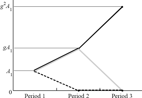
If the bubble does not burst it is assumed to grow at rate g* so that:[4]

where g = 1 + g*.
The possible time paths of the bubble are shown in Figure 1.
Having observed that a bubble has emerged in period 1, the task for the central bank is to minimise the sum of the expected squared deviations of inflation from the target. Since the central bank cannot affect the current rate of inflation, this amounts to minimising:

where E denotes the expected value and subscripts refer to time periods.[5] This objective function assumes that the central bank is not only concerned about the expected value of inflation but also the variability of inflation. This objective function appears to be a reasonable representation of inflation targets in practice. Central banks care about the entire future path of inflation, and they care about the variability of inflation around the midpoint of their target.
We solve the above problem recursively, solving first for the two possible interest rates in period 2; one for the case in which the bubble bursts in period 2, and one for the case in which the bubble continues. Using these solutions we then solve for the optimal interest rate in period 1. This assumes that when setting the interest rate in period 1, the central bank knows that it will be able to change the rate in period 2, depending on whether the bubble has burst or not.
The solutions are analytically quite complicated since non-linearities are introduced by making the probabilities of various outcomes a function of the interest rate.[6] Thus, rather than present the algebraic solution we discuss the solutions for a few different parameter sets. A summary of the results is presented in Table 1.
| Parameter/variable |
Definition |
Case 1 | Case 2 | |||
|---|---|---|---|---|---|---|
| 1a | 1b | 1c | 2a | 2b | ||
| g | Growth rate of bubble | 2.0 | 2.0 | 3.0 | 2.0 | 2.0 |
| ? | Exogenous probability of collapse | 0.5 | 0.5 | 0.5 | 0.2 | 0.2 |
| ? | Effect of interest rates on the probability of collapse | 0.0 | 0.2 | 0.2 | 0.0 | 0.2 |
| ? | Cost of bubble collapse | 2.0 | 2.0 | 2.0 | 2.0 | 2.0 |
| R1 | Interest rate in period 1 | 0.0 | 0.6 | 2.1 | 1.2 | 1.0 |
| p1 | Probability of collapse in period 1 | 0.5 | 0.6 | 0.9 | 0.2 | 0.4 |
| E1(π2) | Expected inflation in period 2 | 0.0 | −1.1 | −3.7 | 0.0 | −0.6 |
| Note: The inflationary effect of the bubble (?) and the initial size of the bubble (A1) are always set equal to 1. | ||||||
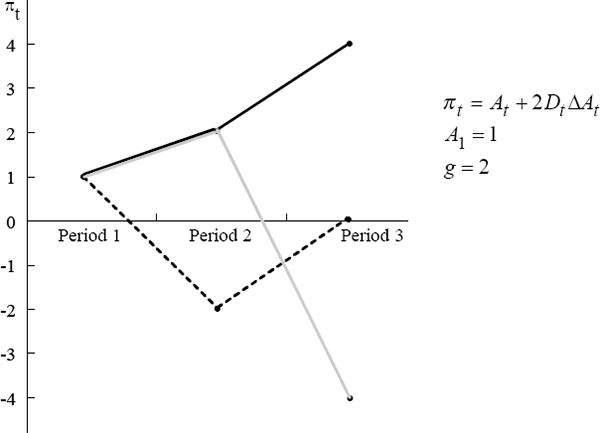
In the following examples we set α = 1 and the size of the bubble in the first period, A1, equal to 1. Initially, we set β = 2; this values implies that the asymmetric effect of asset price changes on inflation is quite pronounced. We also set g = 2 (if the bubble survives, it doubles in size each period). Using these parameters, we illustrate the three possible paths for inflation in Figure 2 assuming that the interest rate is equal to its neutral rate for all periods. If the bubble bursts going from the first to the second period, then inflation is below target in period 2 but then returns to target in period 3. However, if the bubble does not burst going into period 2, inflation is above target in period 2, but more importantly, inflation will necessarily be either substantially above or substantially below target in period 3.
In the next few examples we combine the above parameter settings with the exogenous probability of the bubble bursting next period, ø, set at 0.5. That is, if the interest rate is at its neutral level, the probability of the bubble bursting is 0.5.
Now suppose that changing the interest rate has no effect on the probability of the bubble bursting (φ = 0); this is case 1a in Table 1. In this example the optimal policy is to leave the interest rate unchanged (at the neutral rate); if the bubble continues next period, inflation will equal +2, if it collapses inflation will equal −2. Given that these two events have the same probability of occurring, the expected loss from the bubble bursting is equal to the expected loss from the bubble continuing. Expected inflation is equal to the target in periods 2 and 3. The expectation at period 1 of the sum of squared deviations of inflation from target is 4 and 8 for periods 2 and 3 respectively. This ‘variance’ cannot be reduced by changing the interest rate.
In this example, monetary policy cannot affect the probability of the bubble bursting and so possible events beyond the standard transmission lag (one period) have no bearing on the current setting of policy. Of course, possible events next period are important; if we increase the growth rate of the bubble, reduce the probability of the bubble collapsing, or reduce the costs associated with a bubble collapse, interest rates should be increased, rather than held constant.
Now instead, suppose that the central bank can affect the probability of the bubble
bursting (say φ = 0.2). In this case (1b in Table 1) the optimal policy
is to raise the interest rate by 0.6 above the neutral
rate.[7]
The higher interest rate increases the probability of the bubble collapsing
from 0.5 to 0.6. The effect of this policy is to cause expected inflation to
be below target in the second period (expected inflation will be at the target
in the third period). Even though expected inflation is below target, the expected
squared deviations of inflation from target is actually lower for periods 2
and 3 combined (that is,  .
.
Where does our result come from? Monetary policy has two effects in this model: one standard and one non-standard. First, if the central bank takes the probability of the bubble collapsing as fixed, it faces the usual problem of making decisions under uncertainty. The bank solves this problem by determining the possible levels of inflation in the second period and then, taking the relevant probabilities as given, solves for the interest rate that minimises the expected variance of inflation around the target. The expected rate of inflation is equal to the bank's target.
The second, and non-standard, effect of monetary policy is on the probability of the bubble collapsing. If the central bank can affect this probability, it needs to take into account not only possible outcomes in period 2, but also possible outcomes in period 3. While the standard transmission lag is only one period, monetary policy can affect the probability of events occurring in subsequent periods. If policy can burst the bubble in period 2, the probability of the bubble bursting in period 3 is reduced to zero (because the bubble does not re-emerge). In this example, it makes sense for the central bank to raise the interest rate to increase the probability of the bubble bursting in period 2 and thereby reduce the probability of an even more extreme outcome in period 3.
As the growth rate of the bubble increases, the optimal interest rate increases at an increasing rate. A higher growth rate of the bubble increases the variance of possible outcomes in each of the following periods, with the effect being substantially larger for the third period. As a result, the pay-off to bursting the bubble in period 2 rises. For example, if g equals 3 rather than 2 (so that the bubble triples in size each period, rather than doubles), the optimal interest rate in the first period is 2.1 above the neutral level and the probability of the bubble collapsing increases to 0.9 (case 1c in Table 1). In a sense, the large increase in the interest rate amounts to a strategic attack on the bubble. Policy is tightened to such an extent that the bubble will almost certainly break. The policy-maker knows that this will be quite contractionary; not only will growth be retarded by the lagged effect of the high interest rate, but it will also be adversely affected by the flow-on effects of the fall in asset prices. Yet failing to increase the interest rate results in a much higher probability of a larger crash at some later point.
In case 1a above, optimal policy involves maintaining the interest rate at its neutral rate when the probability of the bubble bursting is exogenous, but increasing the interest rate when the probability is endogenous. We now consider case 2a, in which the optimal policy is to increase the interest rate when the probability of the bubble bursting is exogenous. To do this we reduce ? (the exogenous probability of collapse) from 0.5 to 0.2, while keeping all other parameters unchanged. With a reduced probability of the bubble bursting next period, it is more likely that the inflation will be above target in the second period and so the optimal interest rate in period 1 is higher than it was in the earlier case (1.2 compared to 0). If we now make the probability of collapse endogenous (φ = 0.2), the optimal policy again sees the interest rate above the neutral level (to 1.0; case 2b), but the interest rate is smaller than that required when the probability of collapse is not influenced by monetary policy.
In this example, the higher interest rate needed to counteract the expansionary effect of the asset-price bubble also increases the probability of the bubble collapsing; this amplifies the expected effect of the tightening of policy. The central bank should therefore increase the interest rate by a smaller amount than would otherwise be the case. This result comes partly from the way we have modelled the probability of the bubble collapsing (Equation 2). If this probability is a function not of the deviation of the interest rate from the neutral level, but of the difference between the interest rate and the rate needed to offset the standard expected demand effects of the bubble (1.2 in the above example), then monetary policy would always be tightened by more than the standard analysis would suggest.
While the results described so far are partly driven by the value of parameters that we have chosen, the basic insight of the model is general and holds true for a wide range of parameter values. The fundamental point is that the central bank may need to raise interest rates to attempt to burst an asset-price bubble with the result that expected inflation is below target in the short run. This conclusion is driven by three basic elements of the model. Namely, that the probability of the bubble bursting is an increasing function of the interest rate; that if a bubble bursts it does not return (in the near term) and that the central bank has a desire to avoid very extreme deviations of inflation from target. This result will hold for some range of parameter values, so long as either one of ?, the direct effect of the bubble, or ?, the indirect asymmetric effect of the bubble collapsing, are non-zero.
3.2 A Simple Extension – Bigger Bubbles are More Likely to Burst
We have assumed that the probability of the bubble bursting in the next period is only a function of the current interest rate. This can be generalised to allow for other influences on this probability. Here we allow the size of the bubble to affect the probability of it bursting next period. We assume that the larger is the size of the bubble the higher is the probability that the bubble will burst in the next period. This assumption can be justified on the grounds that as the bubble becomes larger and larger, more and more people identify the increase in asset prices as a bubble and become increasingly reluctant to purchase the asset; this makes it more likely that a correction will occur.
To capture this idea we replace Equation (2) with the following:

We again consider the solutions when the initial size of the bubble equals 1, the growth rate of the bubble is equal to 2, the exogenous probability of collapse equals 0.5 and the effect of interest rates on the probability of collapse equals 0.2 (this is case 1b above, with ? equal to zero). We begin by assuming that ? is equal to 0.15 (case 3a in Table 2). By allowing the probability to be influenced by the level of the bubble, the optimal interest rate response is reduced. In this example, the optimal interest rate in period 1 is 0.3, rather than at 0.6. If we increase the impact of the bubble's size on the probability of the bubble bursting, interest rates may actually fall below the neutral rate (case 3b). The intuition is that if it is likely that the bubble will collapse under its own weight, the case for monetary policy to be used in an attempt to burst the bubble is much weaker. If there is a high probability that the bubble will burst of its own accord, monetary policy needs to be more concerned with the contractionary effects of the expected collapse; in some circumstances this might require a reduction in interest rates before the collapse actually occurs!
| Parameter/variable | Definition | 1b | 3a | 3b |
|---|---|---|---|---|
| g | Growth rate of bubble | 2.0 | 2.0 | 2.0 |
| ? | Exogenous probability of collapse | 0.5 | 0.5 | 0.5 |
| ? | Effect of interest rates on the probability of collapse | 0.2 | 0.2 | 0.2 |
| ? | Effect of bubble size on the probability of collapse | 0.0 | 0.15 | 0.3 |
| ? | Cost of bubble collapse | 2.0 | 2.0 | 2.0 |
| R1 | Interest rate in period 1 | 0.6 | 0.3 | −0.1 |
| p1 | Probability of collapse in period 1 | 0.6 | 0.7 | 0.8 |
| E1(π2) | Expected inflation in period 2 | −1.1 | −1.2 | −1.1 |
| Note: The inflationary effect of the bubble (?) and the initial size of the bubble (A1) are always set equal to 1. | ||||
3.3 Rational Expectations
In our model we do not allow the current size of the bubble to be influenced by the current interest rate, nor do we allow the growth rate of the bubble to be influenced by the level of the interest rate. In this regard, the behaviour of the asset-price bubble in our model is not entirely satisfactory. More generally, the behaviour of the bubble is not consistent with rational expectations. However, we argue that it is not possible to incorporate rational expectations into our model. Even so, we believe that our model provides a realistic description of how a central bank should respond to asset-price bubbles.
For a bubble to satisfy the requirements of rational expectations, the expected capital gain on the bubble component of the asset must be equal to some given outside rate of return (Blanchard and Fisher 1994). In the case of a deterministic bubble, the bubble expands at a fixed rate. In the case of a stochastic rational bubble, there is some probability that the bubble will collapse, so that the growth rate of a surviving bubble is higher than the growth rate of the deterministic bubble. This difference is necessary to encourage rational investors to hold the asset. In fact, the growth rate of a surviving bubble must increase when the probability of the bubble collapsing increases.
In our model, there is some probability that the bubble will collapse. However, the growth rate of a surviving bubble is independent of this probability.
Before explaining why it is difficult to incorporate rational expectations in our model, we present a familiar example of the relevance of rational expectations for monetary policy and asset prices. In the Dornbusch (1976) model of exchange rate overshooting there are two broad effects on the exchange rate of a surprise tightening of monetary policy that causes domestic interest rates to rise above the foreign interest rate. First, uncovered interest parity says that the expected exchange rate must be depreciating – that is, the growth rate of the exchange rate has fallen. Second, when the tightening is announced, the level of the exchange rate will jump. In this model the size of the initial exchange rate appreciation is determined by the final equilibrium level of the exchange rate and the speed of adjustment along the path to the final equilibrium.
Compare this to the effect of an increase in the interest rate on an asset-price bubble. The return on the bubble component of the asset price is equal to the expected capital gain on the bubble, which we take as given. When the interest rate increases, so does the probability of the bubble bursting. Therefore, to keep the expected capital gain on the bubble constant, it must be the case that the growth rate of a surviving bubble increases. However, the value of the asset-price bubble should also have a discrete jump down when the interest rate increase is announced. Unlike the example of exchange rate overshooting, there is no way of tying down the size of the initial jump in the bubble when the interest rate changes. This is because the size of the bubble is indeterminate in the first place, given that the bubble by definition is a deviation from the fundamental value of the asset. Herein lies the problem of incorporating rational expectations into our model.
A naive approach would be to make the growth rate of a surviving bubble (g*) an increasing function of the interest rate. By itself this could imply a circumstance where the central bank would actually want to lower interest rates in order to reduce the size of a surviving bubble! A more complete analysis would be likely to rule out this prescription by realising that there would be a discrete jump in the level of the bubble in the opposite direction of the interest rate change (for a large enough increase in interest rates the bubble may even collapse instantaneously).
If we are primarily concerned with property prices, the failure of rational expectations in our model is not a major issue. Changes in interest rates do not appear to lead to immediate and discrete jumps in the level of property prices, as might be the case for other assets which are continuously traded in relatively deep markets.[8] We regard it as a realistic assumption that the central bank takes the current level of property prices as given and that a change in interest rates does not lead to an immediate jump in property prices, but does increase the probability of the bubble bursting.
3.4 A Summary
The above discussion highlights a number of general points:
? A central bank may wish to raise interest rates to increase the chance of an asset-price bubble bursting in the short run if declines in asset prices have significant effects on the stability of the financial system. While such a policy is likely to lead to a period of below trend growth and inflation below target in the short run, it reduces the probability of the much larger medium-term swings in output and inflation that would eventuate if the bubble was allowed to continue unchecked.
? The monetary authorities need to be concerned with possible outcomes beyond the period of the normal transmission lag. If the probability of a bubble collapsing is endogenous, the expected path of the economy beyond the control lag is affected by today's interest-rate decision.
? If interest rates need to be increased to offset the standard expansionary effect of a bubble, the size of the optimal interest-rate increase may be smaller if the probability of a bubble collapsing is endogenous rather than exogenous. By adding what amounts to an additional transmission channel, the size of the optimal response may decline. Also, the case for higher interest rates is weakened if there is a high probability that the bubble will collapse under its own weight.
Footnotes
Equation (1) relates the inflation rate of goods and services to the level of asset prices, rather than the inflation rate of asset prices (which would be more natural). However, given the fact that we are only concerned with three discrete time periods we ignore any distinction between shifts in the price level and inflation. [2]
In addition, a decision by the central bank to increase the interest rate could be accompanied by remarks regarding the high level of asset prices and the unsustainability of current trends; such remarks might also make the continuation of the bubble less likely. [3]
Our model is not consistent with rational expectations. In a world of rational expectations, monetary policy induced interest rate changes will not only affect the probability of collapse, but also the current size of the bubble and the growth rate of a surviving bubble. We discuss the relevance of rational expectations in more detail below. [4]
In period 2, the objective becomes to minimise  .
[5]
.
[5]
The analytical solutions were derived with Mathematica Version 3.0. [6]
The units are not important here, as they could be rescaled by introducing a parameter on the interest rate in Equation (1). [7]
Although, discrete jumps in property prices could be partially obscured by the fact that data on these prices are not collected on a continuous high-frequency basis. [8]