RDP 2001-08: City Sizes, Housing Costs, and Wealth 3. The Distribution of City Sizes
October 2001
- Download the Paper 163KB
3.1 Zipf's Law
Australia's apparently more expensive housing does not seem to be due to differences in government policy or household preferences. An alternative candidate explanation for the importance of housing wealth in Australia is that the urban population is concentrated in two large cities with relatively high housing costs. In most developed and many developing countries, the population size and population ranks of cities are distributed approximately according to a power law. This means that if a country's urban centres are ordered by population size, the rank of city S (largest = 1, second-largest = 2, and so on) has an inverse relationship with its population p(S):

where a and ζ are positive constants. This empirical regularity can be demonstrated graphically by plotting the natural logarithm of the rank of each city against the natural logarithm of its population size. Figures 2–4 show this relationship for a range of developed and developing countries. When the exponent ζ equals 1, this empirical regularity is known as Zipf's Law (Zipf 1949), corresponding to a slope of –1 for the lines in these figures.[8]
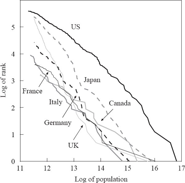

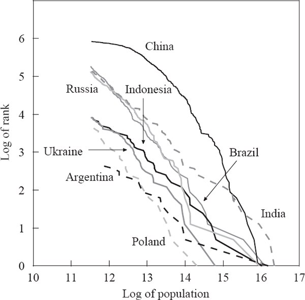
Some empirical support for Zipf's Law has been shown for US cities through time (Krugman 1996; Ioannides and Dobkins 2000), while international evidence has been more mixed (Kamecke 1990). Recent literature on this power law has presented OLS estimates of the slope of this ‘Zipf curve’ as evidence of the exponent ζ being 1. Although OLS is not an ideal estimation method when the left-hand side variable is the log of an integer, maximum-likelihood estimates give similar results (Kamecke 1990; Urzúa 2000).[9]
Although the evidence is mixed, a power law seems to be a reasonable first approximation of the data for many countries. In contrast, models of city formation based on economic first principles such as the location decisions of workers and owners of capital have generally failed to capture the size distribution seen in the data. For example, Henderson's (1974) model could only generate city sizes that varied at all by introducing different traded-goods industries facing (unexplained) differences in production-function parameters; there was no mechanism for generating the observed power law except by assumption. It would be equally misguided, however, to develop a theory that could only generate a Zipf-type power law distribution.
As indicated in the figures above, the rank-size relationship of Australian cities differs noticeably from the predictions of Zipf's Law, and the relationships seen in other countries. This is confirmed by estimates of the power law exponent (ζ) for different countries (Table 6). The point estimates for Australia using either estimation method are below that for all the other countries except China, which has a city-size structure completely different from a power law. The plot of log rank against log size for China is nowhere near linear, for reasons we can only speculate about.
| Zipf curve exponent estimates | Share of urban population in two largest cities |
Primacy ratio(a) | ||
|---|---|---|---|---|
| OLS | MLE | |||
| Argentina | 0.68 | 0.80 | 68.7 | 8.92 |
| Australia | 0.62 | 0.71 | 54.2 | 1.18 |
| Belgium | 0.92 | 1.28 | 47.7 | 1.44 |
| Brazil | 1.22 | 1.19 | 26.8 | 1.77 |
| Canada | 0.82 | 0.82 | 42.6 | 1.35 |
| China | 1.08 | 0.56*** | 4.6 | 1.11 |
| France | 0.98 | 0.92 | 48.8 | 7.38 |
| Germany | 1.28 | 1.31 | 20.0 | 2.04 |
| Indonesia | 0.89 | 0.82 | 35.1 | 3.39 |
| Italy | 1.14 | 1.31 | 27.1 | 1.96 |
| Japan | 1.32 | 1.21 | 15.2 | 2.43 |
| Netherlands | 1.24 | 1.28 | 28.0 | 1.02 |
| New Zealand | 0.74 | – | 59.1 | 2.97 |
| Poland | 1.31 | 1.39 | 21.4 | 1.97 |
| Russia | 1.18 | 1.06 | 19.0 | 1.97 |
| Spain | 1.32 | 1.36 | 28.0 | 1.86 |
| Ukraine | 1.11 | 0.96 | 20.9 | 1.64 |
| United Kingdom | 1.83 | 2.23** | 19.0 | 6.90 |
| United States | 1.01 | 0.76** | 15.7 | 2.04 |
|
Notes: MLE estimates exclude New Zealand due to insufficient number of cities.
**,*** indicates related Lagrange multiplier test of ζ = 1
rejected at 5 per cent and 1 per cent significance levels. Sources: See Appendix B |
||||
Australia's low ζ implies that city populations are lower further down the rank ordering than Zipf's Law predicts. Indeed, Australia has no middle-sized cities according to the UN definition of between 500,000 and 1 million inhabitants. In 1999, Newcastle, the sixth-largest had around 480,000 residents and Adelaide, the fifth-largest city had 1.09 million. By contrast, Australia's small towns follow Zipf's Law very closely: estimates of ζ for the set of towns with populations between 5,000 and about 80,000 are very close to 1. This suggests that population growth behaves in roughly the same way across Australia's small towns, but that small towns as a group behave differently from large towns and cities. The result is surprising, given that the literature finds that Zipf's Law usually holds in the upper tail of the city-size distribution (Gabaix 1999b).
Why does Australia have so few middle-sized cities, resulting in such a low ζ in the upper tail of the city-size distribution? One circumstance where the estimated Zipf coefficient could be lower than 1 is where smaller cities had lower average growth rates or higher variances of their growth rates than the larger cities. A lower mean growth rate could occur if natural population increase is roughly the same nationwide, but larger cities systematically attract residents away from smaller cities. Similarly, smaller cities might have narrower industrial bases and thus be more susceptible to industrial shocks, leading to population growth having a higher variance than in larger cities (Gabaix 1999b).
3.2 The Primate City and Deviations from Zipf's Law
Models of the development of city sizes based on random growth from a common distribution can explain the rank-size rule observed in the population structures of many countries. However, other countries have only one significant city, or a city that is much larger than would be expected based on the Zipf power law. In the geography literature, these are referred to as primate cities (Jefferson 1939).[10] Zipf's Law predicts that the largest city in a country should be double the size of the next largest – a good approximation for many countries. In countries with primate cities, however, it can be six to eight times as large as the next-largest city, and well out of line with the power law describing the relative sizes of the smaller cities in that country. The primacy ratio is the ratio of the largest to the second-largest city. If Zipf's Law holds, this primacy ratio should be around 2; if it is above 3, the largest city is considered a primate city.[11]
Australia is often considered to be a country with no primate city. It is certainly true that Sydney's population is substantially less than twice that of Melbourne. Even if Newcastle, Wollongong and the Central Coast are included in Sydney's population as a single conurbation, Sydney's population is well below what would be predicted from the rank-size relationship of the other cities.
One plausible view of Australia's urban structure is that each state capital is a primate city for its state, and that its population size relative to other state capitals is less relevant. Hill (1974) demonstrated that if the cities in each region of a country follow Zipf's Law, then the rank-size relationship for the whole country will also be approximately consistent with Zipf's Law. As mentioned earlier, the rank-size distribution for Australian towns with fewer than 80000 inhabitants – that is, smaller than Hobart, the smallest of the state capitals – is close to that predicted by Zipf's Law, but larger cities have a flatter rank-size relationship. This is consistent with Australia's nationwide rank-size relationship being a combination of several state rank-size relations where the largest city is a primate, while all the others follow Zipf's Law. It also clearly suggests that smaller towns are subject to random growth of a common nature, while the state and national capitals evolve according to different forces.
Canada also has a relatively flat rank-size curve and a federal political system. Provincial capitals tend to attract residents from other parts of the province because their positions as the seat of government results in these cities offering employment opportunities in administration and policy that are not available elsewhere.[12] Unlike Australia, the provincial capitals in Canada are not usually the largest cities in the provinces. This may help explain both why Canada's Zipf curve is not as flat as Australia's, and why dwelling prices are lower there; demand pressures on housing from internal migration will be spread over two cities in each province – the economic centre and the political centre. The difference may reflect the history of colonisation by European settlers, and this may help explain the current urban structure.
Because both these countries have relatively small populations spread over a large area, transport costs and political institutions may have induced multiple centres of economic activity, resulting in the formation of a primate city for each region. In more densely populated countries such as the United Kingdom, transport costs are less important. A single primate city may arise in those countries, but there may be little impetus for others to form, as centralised administrative functions can cover the entire country, without subsidiary regional centres to cover some areas. Ades and Glaeser (1995) found that a relative lack of transport infrastructure tended to foster centralisation into large cities. Sparsely populated countries such as Australia and Canada have fairly sparse transport infrastructure relative to more densely populated developed countries. This may be encouraging the relatively high concentration of these countries' populations into a few cities, albeit on a regional rather than national basis.
3.3 Implications of the Urban Structure for Dwelling Wealth
As a rule, primate cities account for a greater fraction of the total population than would a largest city that followed Zipf's Law. Larger cities tend to have more expensive housing than smaller cities, so the national average housing price will be higher as the primacy ratio rises, even if housing prices in individual cities are unaffected by this change. Holding national population fixed, an increase in the primacy ratio (or the concentration of population in the largest city) reduces both the absolute population and relative share of the other cities, which may be expected to reduce their average housing prices. Nonetheless, the national average housing price will rise if the population share of the largest city rises, given reasonable assumptions about the functional form of the relationship between population and housing prices at the city level.[13] This implies that if a primate city exists, or more generally, the population is concentrated in a few large cities, national average housing costs tend to be higher than would be true if Zipf's Law held.
How important is this urban structure effect? Our best guess is that it accounts for about one-third of the difference between the dwelling wealth-income ratios of Australia and the United States. Although this estimate is necessarily rough, we believe it conveys the correct order of magnitude, if not the exact figure.
Recall Figure 1 in Section 2.3, which showed housing price-income ratios for individual cities in Australia and the United States. Other than Sydney, the ratios for Australian cities are only somewhat above the average value for US cities of comparable size, and just above the bounds of US experience.We estimated a line of best fit for housing price-income ratios in US cities, given their populations (this is the trend line shown on Figure 1). We used the fitted values to derive the price-income ratios they implied for cities equal in size to each of Australia's major cities. Multiplying these ratios by a measure of income for each city, comparable to those used in the disaggregated US data, gives a counterfactual price for Australian housing (Table 7). These are the prices that would prevail in Australia if the US relationship between city size and price-income ratios also applied to Australia.
| City | Actual house prices | Counterfactual house prices |
|---|---|---|
| Sydney | 6.68 | 3.21 |
| Melbourne | 4.24 | 3.15 |
| Brisbane | 4.75 | 2.92 |
| Perth | 4.72 | 2.87 |
| Adelaide | 4.27 | 2.80 |
| Canberra | 3.35 | 2.49 |
| Hobart | 3.31 | 2.34 |
|
Sources: See Appendix B |
||
The counterfactual prices can be aggregated along with actual data for non-metropolitan housing prices, to derive a national average dwelling price and thus a counterfactual ratio to disposable income comparable to the figures in Table 2.[14] The difference between this counterfactual price-income ratio and the US figure in Table 2 represents the urban structure effect – the part of the difference between the two countries' ratios attributable to the greater concentration of Australia's population in larger, more expensive cities. As shown in Table 8, the counterfactual ratio of price to disposable income for Australia is 2.29, implying that the urban structure effect accounts for around one-third of the gap between the US and Australian ratios.
| Data |
Ratio to survey-based median gross household income | Ratio to national accounts average household disposable income |
|---|---|---|
| US actual data (Flow of funds housing prices, 1997) | 2.76 | 1.63(a) |
| US actual data (Realtors housing prices, 1997) | 2.93 | 1.72 |
| Australian actual data | 5.01 | 3.55(a) |
| Australian counterfactual data | 3.48 | 2.29 |
|
Note: (a) These figures are also reported in Table 2 Sources: See Appendix B. |
||
We have made a number of assumptions on the way to obtaining this estimate. Firstly, we used data on prices for detached houses, not all dwellings, in individual US cities from the National Association of Realtors (NAR). Although these seem roughly comparable with the data underlying the flow of funds wealth estimates, we cannot be sure how different they are. However, the difference between average detached house prices and total dwelling prices in Australia is not large, so this probably does not make much difference to the estimated urban structure effect.
Secondly, the non-metropolitan house price data for the US and Australia are not strictly comparable. The NAR does not publish data for non-metropolitan homes (those located in cities with less than 100,000 inhabitants), so we assume a ratio of price to gross income of 1.5 for non-metropolitan areas to derive the national averages shown in the second row of Table 8. This figure seems reasonable: it is roughly comparable with the price-income ratios of the smallest cities in the NAR data and the national accounts estimate in Table 2. However, we cannot make this assumption for non-metropolitan houses in Australia. The non-metropolitan Australian price data (the CBA/HIA's ‘Rest of State’ series) is highly aggregated and does not distinguish between regional centres (with populations over 100,000) and small towns. Consequently, we use the actual data for the non-metropolitan prices, making the counterfactual a statement about capital-city dwelling prices.[15]
Thirdly, US data on household income by city is from the Current Population Survey which, like Australia's Household Expenditure Survey, reports lower income than the national accounts. The data are also only available as median gross income, not average disposable income. Cross-country differences in the gap between survey measures of income and the national accounts are therefore built into our estimate of the urban structure effect, perhaps inflating it.
Of course, this estimate assumes that the average price-income ratio for cities of the same absolute size is the appropriate basis for cross-country comparison, and that the level of dwelling prices in the US is at an equilibrium. Relative city sizes clearly matter for housing costs within countries, but without city-level dwelling price and income data for a wider range of countries, we cannot say whether dwelling prices vary with absolute population or relative rank. If cities in different countries with the same rank should have the same price-income ratio, given preferences and other factors, then we should compare Sydney with New York or Los Angeles, not Houston or Atlanta, as we have effectively done in this paper. In that case, the counterfactual price-income ratio for Sydney would be much closer to the actual value, and our estimate of the urban structure effect would be closer to half the gap between the US and Australian data.
Footnotes
Gabaix (1999b) showed that cities with populations that grew randomly would converge to a distribution matching Zipf's Law (ζ = 1) in its upper tail, provided that the growth rates for all cities were drawn from a statistical distribution with the same mean and variance, and that the cities were bounded to be above some minimum size. The existence of such a common distribution is called Gibrat's Law. If this is not true, then Zipf's Law does not hold; Zipf's Law should therefore be seen as a diagnostic for the underlying growth process, rather than a law that must hold in all cases and at all times. Earlier work on explaining Zipf's Law centred on variations of this requirement for random growth from a common distribution. Simon (1955) developed a simple model with additions to the population attaching to existing cities with probability equal to its share of total population. Hill (1974) formalised this proportionality of probability to population as a Bose-Einstein occupancy problem. Gibrat's Law has also been used to study the size distributions of firms, income distributions and other economic variables; see Sutton (1997) for a review. [8]
The OLS estimates are based on an inappropriate specification of the errors, so their standard errors and t-statistics are not meaningful and we have not reported them here. The residuals for both sets of estimates have a cyclical pattern; similar-sized cities tend to have residuals of the same sign. Explaining this is beyond the scope of the paper, but it suggests that there is more to the city-size distribution than a simple power law. [9]
Countries with obvious primate cities include Argentina, Denmark, Finland, France, Greece Indonesia, Norway and the United Kingdom. [10]
Thresholds for defining primate cities have evolved over time. Jefferson's (1939) original definition of a primate city was one that was more than twice as large as the next-largest city, that is, any upward deviation from Zipf's Law. [11]
These opportunities are in addition to the normal range of private-sector occupations seen in a city of that size, rather than a substitute for them. By contrast, manufactured political capitals such as Brasilia, Canberra or Islamabad have narrower employment bases focused on the public sector. This may explain why these capitals do not become primate cities. [12]
In particular, this will hold if house prices in individual cities are a rising function of population with a second derivative that is always non-zero; a proof of this is available on request. The result also holds for some cases where h” = 0 at some point. [13]
To be consistent with the data in Table 2, the weights used to aggregate the city data are slightly different from the population data used in Section 3.1. We also use 1998/99 data for Australia, not the 2000 data shown in Figure 1. [14]
This might introduce some upward bias to our counterfactual national average if actual prices are higher than the average US income ratios would suggest. However, we do not have separate price series for these cities, so we cannot tell how important this is. [15]