RDP 2012-08: Estimation and Solution of Models with Expectations and Structural Changes Appendix A: The Kalman Filter Equations

Take the state equation

and the observation equation

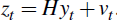
Define and

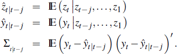
The recursion begins from ŷ_1|0 with the unconditional mean of y₁, in our case

where µ is the steady state under the initial structure, that is µ = (I – Q)⁻¹ C and

implies vec 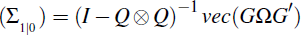. Presuming that ŷ_t|t−1 and Σ_t|t−1 are in hand then

and the forecast error will be

The latter implies that

Next, update the inference on the value of y_t with data up to t as in Hamilton (1994):

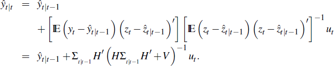
This follows from

after using 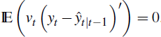. Equation (9) then implies

View MathML

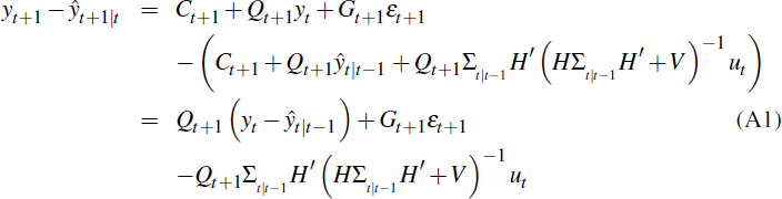
where K_t = Q_t+1Σ_t|t−1 H′ (HΣ_t|t−1 H′ + V)⁻¹ is the Kalman gain matrix.

This last expression, combined with Equation (9), implies that

The associated recursions for the mean squared error (MSE) matrices are given by,

If the initial state and the innovations are Gaussian, the conditional distribution of z_t is normal with mean Hŷ_t|t−1 and conditional variance HΣ_t|t−1 H′ + V. The forecast errors, u_t, can then be used to construct the log likelihood function for the sample as follows:

This is Equation (20) in the text.