RDP 7702: Inflation and Economic Stability in a Small Open Economy: A Systems Approach 3. A Simulation Analysis of Australian Inflation
June 1977
The analysis in this paper is based on simulation of a structural model of the Australian economy. The model is intended to reflect the major mechanisms and institutional features of the Australian economy; it is discussed briefly in section 3.1 below, and the complete model is set out in Appendix A.[11] Section 3.2 discusses the degree to which the model explains the recent take-off in inflation, and fluctuations in other important variables, and section 3.3 presents some counterfactual simulation analysis. This analysis proceeds by eliminating in turn the various proximate causes of the inflationary take-off, to give an idea of the contribution of each of the impulses listed in the introduction. Section 4 draws together the threads of the simulation analysis, and discusses some ways in which the impulses were interdependent.
3.1 The model: crucial features
A basic feature of the model is its representation of economic processes as reflecting partial adjustment towards a moving equilibrium determined by a set of long run behavioural schedules. Thus, for example, desired consumption is determined by disposable income and interest rates, business fixed investment by adjustment to equate the marginal product of capital with the cost of capital, desired imports and domestic output by sales and price of imports relative to that of domestic output. Actual consumption, investment, imports, output, etc. are in general assumed to adjust towards the desired level with a first order adjustment process, although adjustment is also importantly influenced by the gap between actual and desired levels of buffer stocks. The buffer stocks, consisting of money in the case of households and inventories of goods in the case of firms, allow smoothing of the relevant path in the face of unexpected disturbances, and play an important role in the dynamics of the model.
The actual quantity of each buffer stock is determined residually in the short run, reflecting its role as a shock absorber. Thus, for example, the stock of money is determined as the net outcome of all other private and government decisions, as indicated by equation 18 in the model (see Appendix A). An important feature of the money supply process[12] in Australia since the second world war has been a persistent tendency for bank lending to the private sector to increase more than in proportion to bank deposits; that is, there has been a rising money multiplier for much of the sample period.[13] This is reflected in the equation (no. 14) determining bank lending by a term representing the minimum asset ratio of the banks, and another representing the effect of excess demand for funds, and one of the simulation experiments involves setting the parameter on excess demand to zero, and holding the asset ratio constant.
The wage-price sector of the model (equations 6 and 9) is built around a wage-price interaction which is intended to capture implicitly the effects of past and future price movements. Money wages adjust with a lag to bring real wages into line with the marginal product of labour, while prices adjust to a mark-up over unit labour costs. This specification ensures that the effects of past price changes are built into wages and that wage rises feed in turn into prices (in each case with allowance for movements in productivity). Within the framework of the model, however, information about future price movements is provided by the level of real money balances relative to desired real money balances, and, our results to date suggest there are statistically significant and numerically important direct effects of excess money balances upon price and wage dynamics.[14] In addition, labor market disequilibrium is included in the wage equation, to represent the short run Phillips effect of demand pressure in the labor market.
A further direct effect on wages, which is important in the Australian case, is that of the centralized wage fixing authorities. In Australia, Commonwealth and State arbitration commissions set a range of minimum award wages. The important effect of award wages in wage determination which is found in almost all empirical work in this area for Australia[15] can be rationalized in two ways which have not yet been empirically distinguished. One theoretical rationalization would be provided by a two-sector model in which one sector has its wages determined by a mark-up on awards, with wages in the other sector market determined. The second explanation relies on expectational effects; thus Parkin (1973) suggests that the decisions about award wages are an important part of the wage expectations generating mechanism in Australia, and includes a distributed lag on award wages in an equation for average weekly earnings. In the current model, this approach is modified somewhat, and combined with work on the determinants of award wages. This work suggests that awards are usually adjusted for price changes and for trend productivity growth.[16] In the current model, it is assumed that it is only award wages which are higher or lower than those which would be expected on the basis of price changes and the regular productivity changes which influence market wages. If, for example, real award wages are above the level regarded as normal, then this serves as a signal that market rates should be increased, and vice versa if awards are below normal levels.[17]
The other general feature of the model is the way in which it endogenizes movements in the bond rate and the exchange rate, by the inclusion of policy reaction functions for the relevant variables. Equations 20 and 21 explain an interest rate on government securities and the $US exchange rate respectively, and the corresponding financial quantities (the net value of government securities held by the non-bank sector and the level of international reserves) are determined by the relevant demand functions (equations 12 for government securities and the functions entering the balance of payments identity (no. 17)). The policy reaction functions include terms representing the usual stabilization policy objectives, but also dummy variables representing the timing of the several major changes, particularly in the exchange rate, which have occurred in recent times. As is likely to be inevitable with a jumping peg exchange rate regime, these changes were anticipated to a degree. Hence a further dummy, representing the extent to which exchange rate expectations built up prior to each of the discrete exchange rate changes[18] is influential in the trade equations and in the asset demand functions of the model. There is also an endogenous aspect to exchange rate expectations, represented simply in the model by the exchange rate relative to an “equilibrium” exchange rate calculated from considerations of purchasing power parity.
In contrast to interest rate and exchange rate policy, budgetary policy, as represented by tax rates and real government outlays, is assumed to be exogenous. The deviation of real award wages from trend is also assumed to be exogenous in the model. The distinction between the degree of endogeneity of the different policy instruments is not clear cut however: on the one hand the interest rate and especially the exchange rate equation contain exogenous explanatory -variables; on the other hand, the instruments of budgetary policy, and decisions of the arbitration commissions, react to some extent to economic conditions. The choice of which policy instruments to endogenize in a macroeconometric model is obviously somewhat arbitrary, and reflects partly a judgement about the extent to which the exogenous influences dominate over the sample period. If this was the only criteria the exchange rate would probably be exogenous in the current model, but a further important point is that the exchange rate cannot remain fixed in the face of substantial changes in budgetary or monetary policy.[19] It is therefore necessary to allow the exchange rate to fluctuate if sensible counterfactual simulations are to be constructed and this is the main reason for endogenizing the exchange rate in the model. On the other hand, since even the policy instruments regarde as exogenous in estimating and simulating the model are endogenous to a degree, it is necessary to consider this in a complete analysis in section 4 an attempt is therefore made to allow for the extent to which the variables regarded as exogenous in the simulations in section 3, are endogenous, and interdependent.
3.2 Control simulation against actual changes
The panels in figure 2 provide actual and simulated values since 1970 of proportional changes in real output, prices, international reserves, and the money stock; the unemployment rate; and a measure of monetary disequilibrium. The control solution values are obtained from a dynamic simulation of the model from a starting point in 1966. Simulating changes with a dynamic simulation which allows errors to cumulate provides a rigorous test of a model's tracking ability, and a subjective assessment of the model's performance is “moderate”.[20]
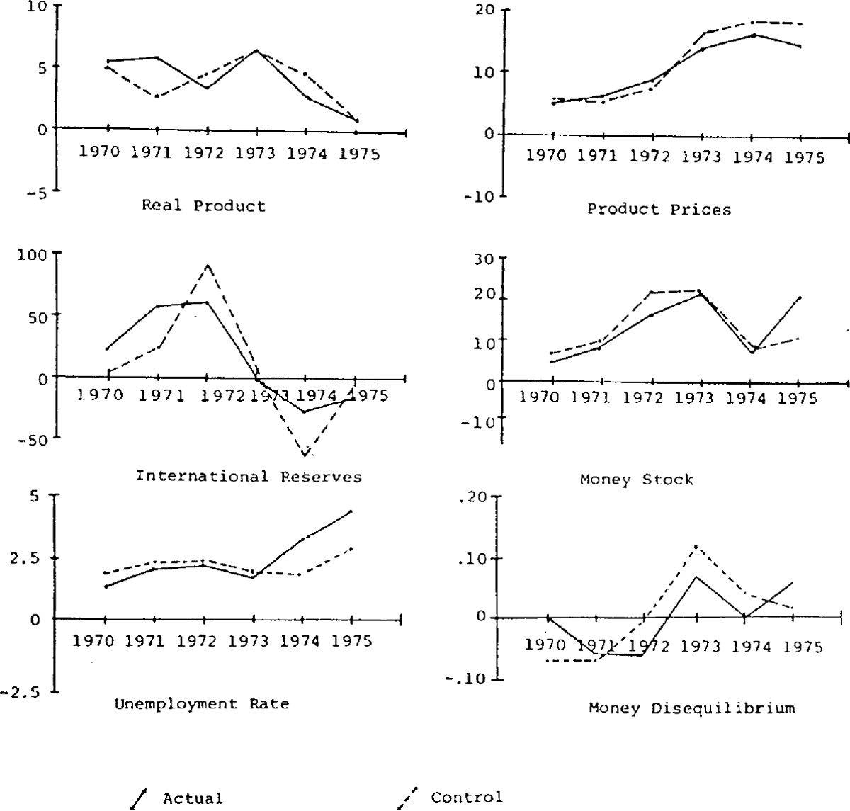
The model's ability to explain levels of each variable is quite high, and the main weakness is the failure to accurately explain short term fluctuations in output and employment. Typically, the model underpredicts output and employment in booms and pverpredicts during slumps, although in the disturbed period in 1970–1972 the timing of output fluctuations is also somewhat astray.[21] In contrast, fluctuations in international reserves are greater in the control solution than in the economy for recent years. The take-off in inflation and the major recent cycle in the balance of payments and the monetary growth rate are explained reasonably well, although the model tends to somewhat over-predict inflation in recent years and the growth in money in 1975 is seriously understated.
The model also captures the major movements in monetary disequilibrium (real money supply less real money demand) reasonably well although the underestimate of the monetary growth rate in 1975 translates into an error in the direction of movement in money disequilibrium. In the control simulation, the supply of money is exceeded by demand in 1970 due mainly to the underprediction of interest rates. This underprediction of interest rates also occurs in 1971 but the effect of this on money demand is offset by the underprediction of real income. The strong growth in unemployment in 1974 and 1975 is not captured by the model, partly due to its aggregated labour market. The wage equation is based on adult male units whereas the equations modelling labour demand and labour supply refer to males plus females and as a result the model tracks movements in the unemployment rate of adult males better than the average for the whole economy,[22] although still not capturing fully the sharp rise at the end of the period.
The point denoted by an asterisk in figure 1 illustrates the control solution trade-off between inflation and unemployment in the model for 1971–1975. As noted, the model somewhat over-predicts inflation and underpredicts unemployment, especially in 1974 and 1975. The underprediction of unemployment is related mainly to the failure to allow for the wage relativity effects mentioned in the last footnote, effects which are virtually impossible to capture in a highly aggregated model.
Despite the imperfect fit of the model it performs well enough to justify its being used for a series of simulation experiments designed to indicate the proximate causes of the inflationary take-off in Australia.
3.3 Some counterfactual simulation experiments
This section presents the results of simulating the model with somewhat different assumptions about the policy regimes and hypothetically removing some of the impulses which impinged in the past six years. Firstly a managed float from early in 1971 is assumed;[23] then a managed float with monetary tightness, achieved by raising interest rates in 1972 and 1973, by fixing bank liquidity ratios and by assuming that bank advances did not there-fore respond to demand, pressures;[24] then a managed float with monetary and fiscal tightness (the previous simulation is repeated with government outlays growing steadily at a slower rate in recent years); and, finally a managed float with monetary and fiscal tightness and with real award wages assumed to grow at a slower rate, corresponding to an assumption that arbitrated wage increases were at a rate which did not raise wage expectations in the labor market. Appendix B specifies precisely the nature of these experiments.
The hypothetical nature of these simulation experiments cannot be stressed too strongly, and there are two reasons why the results should be treated with considerable caution. The first is that the various impulses were not independent, or totally exogenous, as might be thought to be implied by the simulation strategy. Some ways in which the variables assumed to be exogenous were in fact endogenous, and interdependent, are discussed in section 4, and the results of the simulation analysis cannot be considered apart from this discussion.[25]
The second reason for caution in interpreting the results is even more fundamental. As argued by Lucas (1976), since private sector reactions will not be invarient to the policy regime, one cannot be sure that the outcome would be the same as that predicted by the model if different policies had been followed. The methodology of this paper is designed to weaken the force of this objection in two respects. First, the analysis uses a structural model which is designed to enable consequent adjustments to the structure of private sector reactions to be made when the policy regime is altered.[26] Second, the alternative policy regimes are in some respects within the range observed in the sample period: the exchange rate changes under the managed float are less than those which occurred with the variable peg;[27] changing official interest rates and bank cash ratios is a common policy reaction; and the rate at which government outlays and award wages grow in the alternate simulations are similar to those achieved in the latter part of the 1960's.[28] Nevertheless, the issue raised by Lucas is a further reason for caution in interpreting the results.
A managed float
Here the exchange rate reaction function operates without the major revaluations of 1972 and 1973, and the devaluation of 1974. The exchange rate revalues slowly but steadily from 1971 under the influence of the relative price, balance of payments and monetary target variables in the exchange rate reaction function. By the end of the simulation period the rate has revalued slightly more than in the control simulation, but this is achieved without the major revaluations followed by devaluation which occur in the control simulation.[29] Reflecting this, the major fluctuations in the trade account and capital accounts of the balance of payments which occur in the control simulation are absent.
As indicated by figure 3, which compares the control solution with that obtained under the managed float, this removes the major cycle in the balance of payments and the resulting rapid acceleration in the monetary growth rate in 1972 and 1973. Money growth increases from 1973 under the managed float regime, however, because the high domestic credit expansion is not offset by loss of international reserves as in the control solution, and in 1974 and 1975 the monetary growth rate is higher under the managed float.
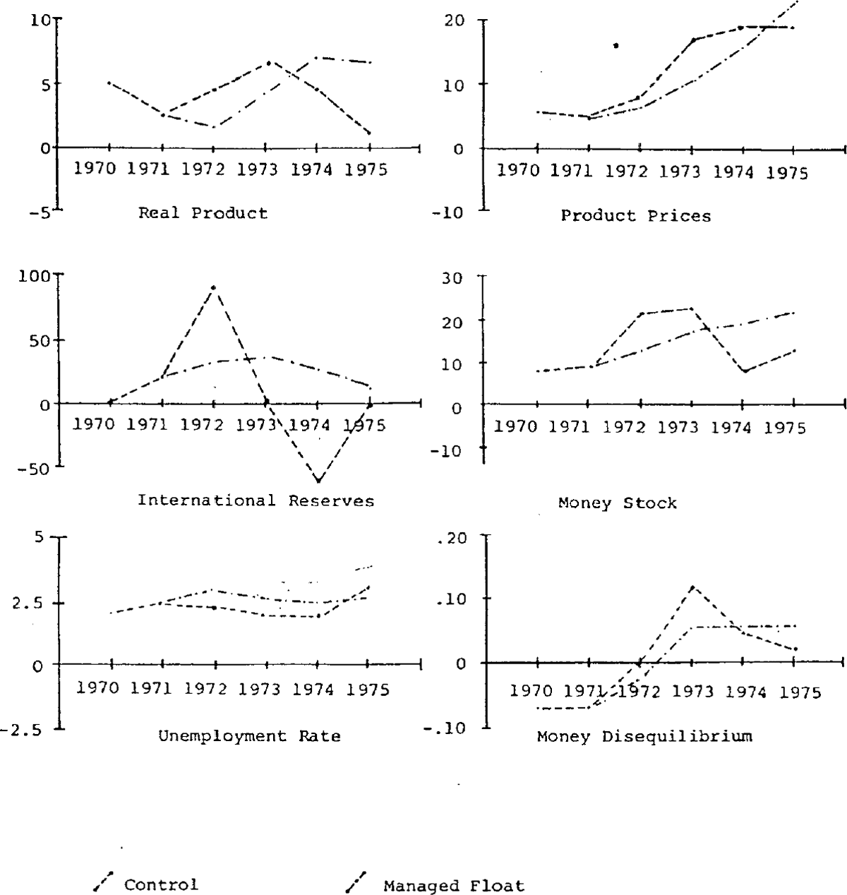
Inflation is less than that in the control simulation, by approximately 7 percentage points in 1973, slightly lower in 1974 and 4 percentage points higher than in the control simulation in 1975, and accelerating sharply. Output growth falls in 1972, as the stimulus provided by expectation of a major revaluation[30] is removed under the assumption of a managed float, but thereafter accelerates steadily to reach an inflationary peak of almost 7 per cent per annum in 1974. The levels of real product and employment are considerably lower in 1973 than in the control solution.
The unemployment rate in this simulation rises above the control solution value in 1972 and remains above until 1974. In 1975 the increased real growth produces a small reduction in the unemployment rate. The influence of the initially reduced growth in international reserves and money is seen in the behaviour of money disequilibrium. The lower growth of money up to 1973 means the inflationary consequences of monetary disequilibrium are lessened considerably. After 1973 however, monetary disequilibrium is greater than in the control solution, largely due to the faster growth in the money supply.
Managed float with tighter money[31]
In this simulation money is tightened by raising interest rates in 1972 and 1973, fixing the bank asset ratio at its initial value, and assuming that bank lending did not respond to demand.[32] This has the effect of reducing the money multiplier and substantially eliminating its rise during the sample period, and increases sales of government securities. As in the previous simulation, a managed float of the exchange rate is also assumed, so that lower domestic credit expansion is not offset by a build up of international reserves, as would tend to occur with a fixed exchange rate.
Examining first the panel depicting monetary growth in figure 4 it can be seen that, with a managed float and tighter money, the money growth rate is about one percentage point less from the beginning of the 1970's, with the major gain occurring towards the end of the simulation period, when monetary growth is reduced by over 4%. International reserves are growing at a slightly greater rate throughout, partly because of the effect of higher interest rates on capital flows, and then the stronger current account. These factors combine to cause money supply to fall by more than money demand, although money demand decreases due to lower real income and higher interest rates. This has strong anti-inflationary consequences, particularly in 1974 and 1975, although at a relatively slight cost in terns of a higher unemployment rate. The rate of inflation is reduced by about a quarter throughout the simulation period, which more than offsets the effect of revaluation on exports and imports. Higher exports and lower imports both contribute to the slightly increased output growth in 1971 and 1972, evident in the first panel of figure 4.
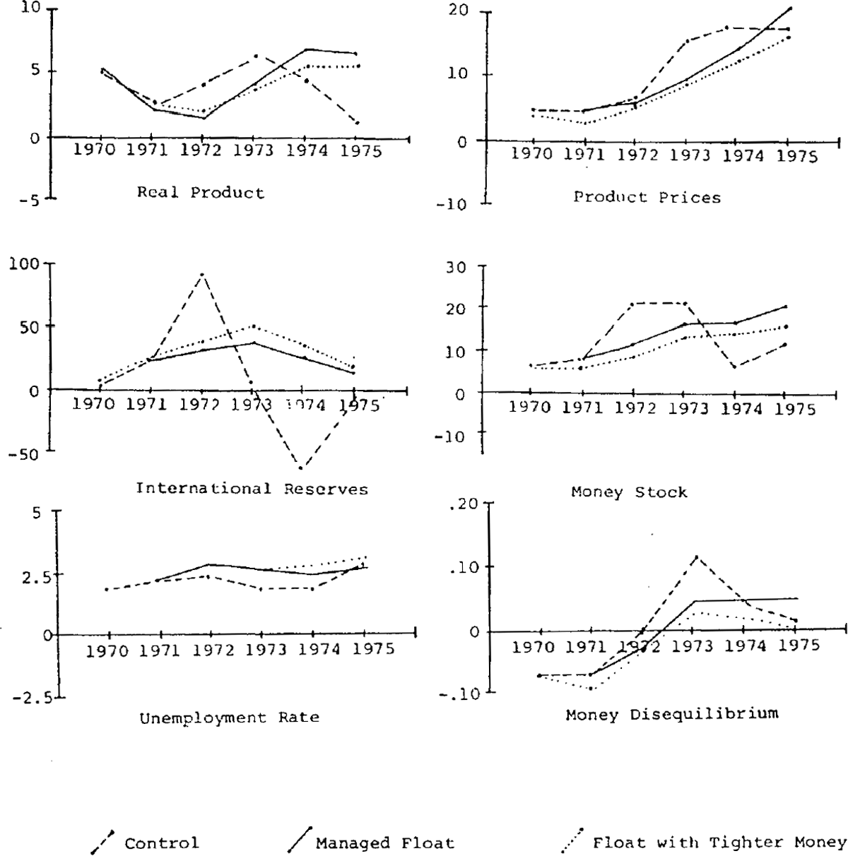
Despite tighter monetary policy and a revaluing exchange rate, prices are still rising (although at a slower rate than in the previous simulation) at the end of the sample period. This is due both to the demand pressures in the goods market, and the effects of the strong wage increases.
Managed float, tighter money and tighter budgetary policy
As noted above, budgetary policy was relatively tight in the early 1970's, then became highly expansionary. Although there were important influences on the revenue side of the budget, these are largely endogenous in the model. On the outlays side of the budget, the growth of government spending on goods and services declined somewhat in the early 1970's and transfers were growing relatively slowly; then transfers expanded strongly from 1971/72 and spending on goods and services from 1973/74. The current simulation, which is compared with the previous one in figure 5, consists of maintaining growth of both spending and transfers, at the rates achieved in the late 1960's, into the 1970's. Thus spending on goods and services is actually higher for a time, then markedly lower.
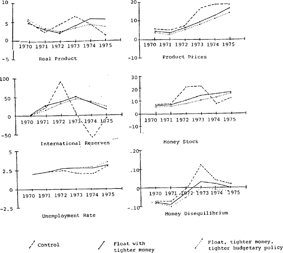
In the simulation, the effect is to produce higher growth in real product until 1973; after that product growth is slightly lower, and unemployment slightly higher; the net effect of a smoother path for real government outlays is smoother growth of real product. Inflation is slightly lower at first, as the effect of higher productivity on unit labour costs offset; the higher degree of demand pressure in the commodity markets; and the cumulative effect of lower prices on the trade account i: sufficient to almost offset the output effect of smaller government outlays late in the simulation period. The monetary growth rate is over 1 percentage point lower at the end of the period, mainly reflecting the lower budget deficits, and the inflation rate is over 2 percentage points lower than in the previous simulation, again largely due to reduced monetary disequilibrium.
Managed float, tighter money, tighter budgetary policy and steady growth of award wages
The final simulation experiment is to remove the large increases in award wages, especially in 1970/71, 1973/74 and 1974/75. This is done with all the other policy changes as in the previous simulation, and so the comparison of the simulation paths illustrated in figure 6 indicates the effect of the large award wage increases.
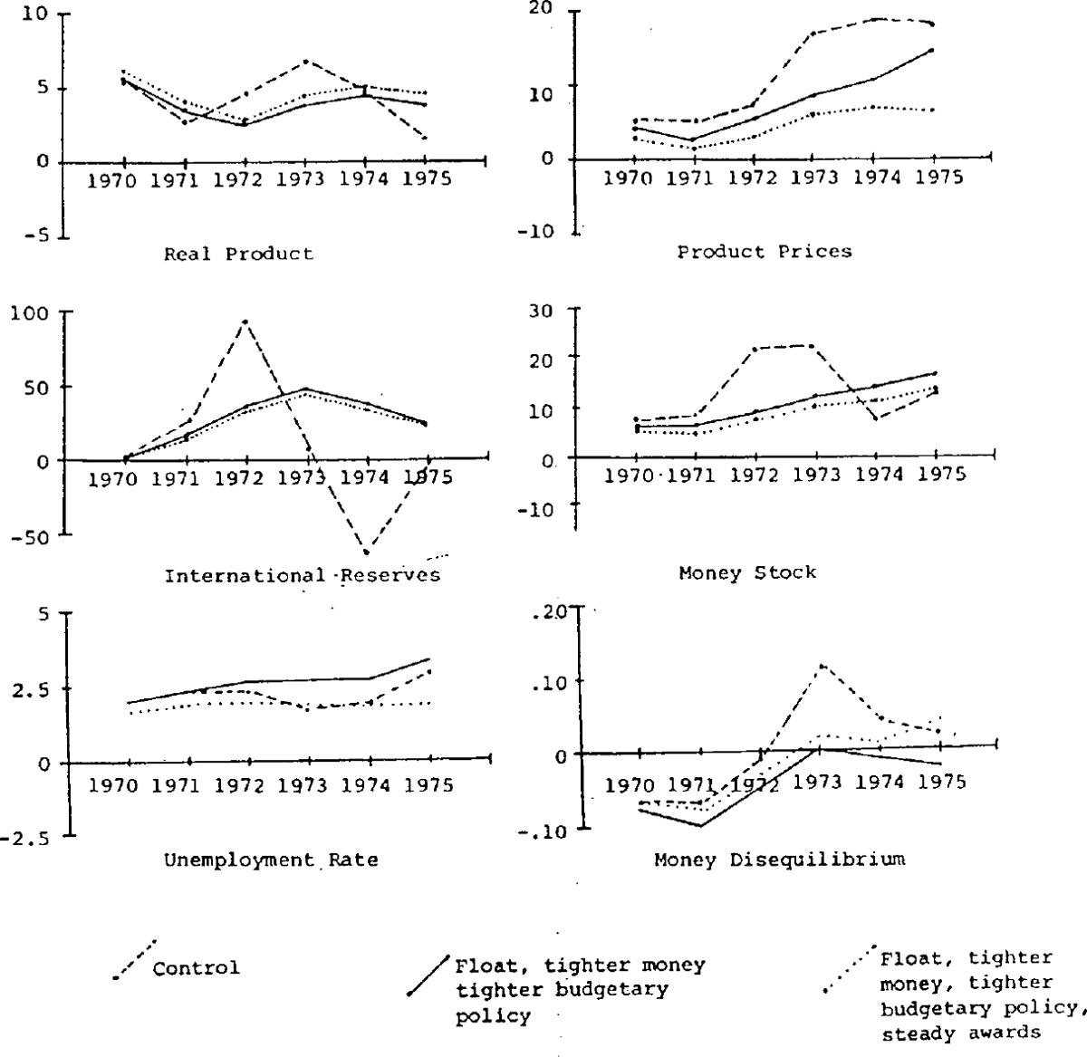
The results of this simulation are similar to those of the previous one, except the inflation rate is lower throughout, and dramatically so in 1974 and 1975. Monetary growth is also substantially lower, reflecting largely the effect of lower wage on government outlays, which is partly but not entirely offset by lower tax collections. An important effect of lower awards, is that unemployment is substantially lower, as a result of lower real wages[33] with higher real output. As might be expected, the tighter monetary and budgetary policies in the previous simulations both reduced employment relative to the control solution values (although the growth of employment is smoother). When the real wage impulse is also removed, in the final simulation, employment is considerably higher throughout, relative to both the previous simulation and to the control solution (except in 1973).
Control solution compared with all variables growing steadily
Comparing the control simulation results with those of the final simulation path, it is evident that removal of the various monetary, budgetary and wages impulses, combined with a managed float, have largely eliminated the dramatic acceleration of inflation which occurs in the control simulation. The slight acceleration of money and inflation in 1973, 1974 and 1975 in the final simulation is because the sizeable revaluation resultin from the managed float is not enough to entirely offset the effects of the massive commodity price rises of recent years. A relatively steady set of policies has produced a smoother output path and a more favourable combination of inflation and employment in the model. This is seen most clearly in the average inflation-unemployment combination for 1971–1975 in the final simulation, denoted by the cross in figure 1; it is interesting that the average trade-off achieved in this simulation is similar to those in the late 1950's and in the 1960's.
This is also indicated by a comparison of the simulation paths in the first and second panels of figure 6, where the growth rate of output is smoother, and higher at the end, and that of prices substantially lower, than in the control simulation. Since real wages are lower in the final simulation, there are favourable employment effects in excess of those indicated by the higher output.
There is still a recession, indicated by the relatively low growth of real product, in 1971 and 1972, partly as a result of the world recession[34] and the revaluation of the $A,[35] and the growth of real product also turns down in 1975, again mainly because of the effects of the world recession on exports. It is evident that the managed float of the exchange rate assumed in the current analysis cannot insulate the economy fully from either sharp fluctuations in world prices, particularly when there are changes in the terms of trade, or from major fluctuations in world activity.[36]
Footnotes
The model is in the tradition of those developed at the International Monetary Research program at the London School of Economics. It is discussed more fully in Jonson, Moses and Wymer (1976). [11]
It should be noted that the model uses a relatively broad (M3) measure of “money”; “credit” is correspondingly defined as bank credit. Future work will investigate alternative treatments which allow for a non-bank credit market in the model. [12]
Until recently, the statutory minimum cash ratio tended to be reduced more or less as the banks ran up against their lending limits, as part of a policy to strengthen the competitive position of the banks. [13]
A comparison of the values of the relevant parameters in equations 6 and 9 when they are estimated with data for different sample periods suggests that they are rising in recent times. [14]
A survey of earlier results is provided by Jonson, Mahar and Thompson (1974); in the current work, the effect of award wages comes through strongly, as indicated by equation 9. The weight of .4 on awards relative to trend is consistent with earlier results suggesting that increases in awards are not fully passed into earnings. [15]
See Jonson, Mahar & Thompson (1974) for the most recent work, and a discussion of earlier results. [16]
As noted above, award wages have recently risen well in excess of historical norms. One of the simulation experiments will involve hypothetically removing this deviation from historical trends. [17]
These exogenous exchange rate expectation effects are set to zero in some simulations in which a more flexible exchange rate regime is assumed. [18]
Unless draconian direct controls are imposed, and even these are likely to be unsuccessful if macroeconomic policy is highly destabilizing. [19]
It is extremely difficult to devise objective tests of the performance of alternative macroeconometric models, as indicated for example, by the discussion of Dhrymes et al (1972). The approximate root mean square percentage errors for key variables in the dynamic control solution of the current version of the model from 1966–1975 are as follows: price of output, 3.9; earnings, 4.4; employment, 1.0; real product, 2.6; international reserves, 13.5; and money, 3.5. [20]
The two problem areas are exports and inventories, where short run movements are not captured particularly well. [21]
Wages and unemployment rates for females and juniors have risen by considerably more than the average for the workforce as a whole in recent years. [22]
In the discussion of the exchange rate reaction function presented above, it was noted that the equation (no. 21) contains both endogenous determinants, such as the level of and changes in the money stock and in international reserves, and the level of prices relative to world prices, and exogenous dummy variables to allow for the timing of the several major changes in parity that occurred. In simulating a managed float, the dummies representing the major changes in parity are set to zero, and the endogenous influences determine the rate. Further discussion is presented below, but it should be noted that a variety of market or policy reaction functions could in principle be substituted to provide alternative ways to simulate a flexible exchange rate. [23]
This represents a somewhat clumsy way to represent a tight money policy within the traditional institutional framework. In practice, it might be more convincing to simulate such a policy by substituting a market reaction function for the policy reaction for interest rates, and by including a market determined bank lending rate, but there are problems of the sort discussed by Lucas (1976) in imposing such a major change of structure on the model. [24]
In principle, this point would be covered by including reaction functions for all the instruments of policy and award wages, and by including some more structural detail in the financial sector of the model. The impulses would be removed by setting to zero those dummy variables which represented the economically exogenous determinants of policy reactions. In practice, knowledge of policy reaction is far too imprecise at present to implement this first best approach. The discussion at the end of section 3.1 is relevant here. [25]
In particular, when a managed float is substituted for the moveable peg exchange rate regime, the dummy variable representing expectations of the once for all changes in the exchange rate (denoted QE) is set equal to zero. [26]
Although it should be noted that there is no example of a managed float during the sample period. [27]
Indeed, the control solution tracks, although imperfectly, with policy and other variables well outside the range in much of the sample period. Jonson, Moses and Wymer (1976) give estimates for the periods to 1971(4) and 1974(4), and it is possible to check the extent to which omitting the highly disturbed observations in 1972, 1973 and 1974 changes the key structural parameters. [28]
In 1975, the rate of revaluation slows, although there is no devaluation, despite the strong expansion of the budget deficit in the last two years. If exchange rate expectations were closely geared to the budget or monetary position this conclusion might be altered, in which case there would be devaluation and increased inflation towards the end of the sample period with the managed float. [29]
Which operates to encourage exports and postpone imports and therefore to encourage domestic production in the control simulation. [30]
In this and subsequent simulations the control solution is plotted as well as the two being directly compared. [31]
Footnote 2 on page 13 explains the reasons for using this approach. [32]
In the short run, lower award wages have a larger effect on earnings than on prices. [33]
World activity is represented in the model by a measure of world trade, which influences the demand for Australian exports. [34]
There is also the depressing effect of a trough in the Australian investment cycle at work. [35]
It is worth noting that a perfectly flexible exchange rate could not insulate an economy from such fluctuations eitnei. [36]