RDP 7903: Monetary Rules: A Preliminary Analysis 3. Simulation Results
September 1979
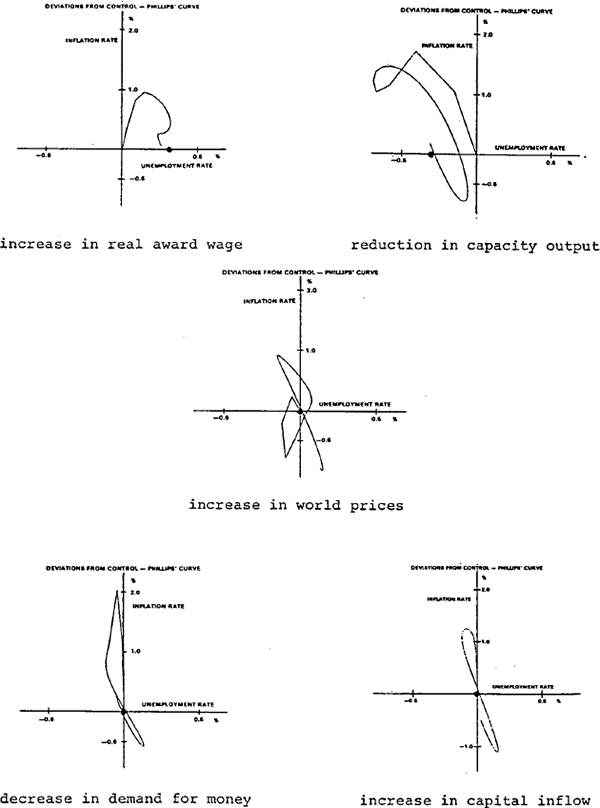
Each of the basic impulses raises the price level. This does not mean that each impulse also expands production or employment, since RBA79 generates a variety of dynamic responses with different impulses. These responses are first discussed in the case of partially accommodating money (i.e. using the estimated policy reaction function for the bond rate) to provide the background which is necessary to evaluate the responses with different regimes for monetary policy. The dynamics are summarised in terms of the Phillips loops of figure 1. More details of the simulations are in the figures of Appendix D.
3.1 The properties of the model with partially accommodating money
The increase of real government spending raises expected sales and aggregate demand. The money supply is initially expanded, while international reserves fall. The additional growth of real product reaches a maximum in the third quarter, at an annual rate of 2 per cent, and then declines quickly. Inflation rises, but by less than the growth of output, reaching a maximum annual increase of .9 per cent after 10 quarters. The impulse sets up a cycle which is damped fairly quickly. Unemployment is reduced by a maximum amount of about .6 of one per cent after 9 quarters. After 7 years, the exchange rate has devalued by around 3 per cent, and the bond rate has risen by 1 per cent. In the steady state, the price level is raised by 5 per cent (a little more than wages), real output is decreased by .1 per cent and unemployment is reduced by .3 of 1 per cent.
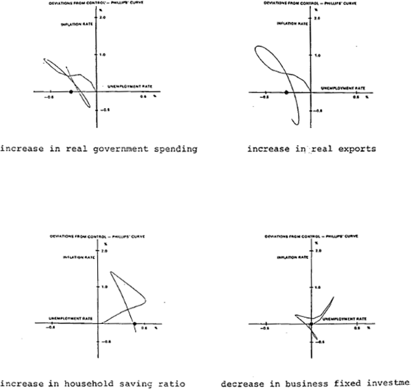
The increase in real exports produces a similar response, except that since the balance of payments strengthens the exchange rate revalues. The initial effect on inflation is larger, and the monetary expansion is greater, than it is when the impulse consists of an increase in government spending. (The difference in monetary response is due mainly to a smaller rise in the bond rate in the case when international reserves increase.) In the long-run the price level falls by 1.6 per cent, wages fall by .5 per cent, real output is raised by 1.8 per cent and unemployment is reduced by .3 of 1 per cent.
When the impulse consists of an increase in the household saving ratio, the growth of real product is initially reduced. The decline in consumption also reduces imports and growth of the mone supply therefore accelerates. With reduced demand for money and increased supply, inflation rises, to reach an annual rate of 1.4 per cent above control after six years.[10] Despite the increase in domestic inflation, the strengthening of the balance of payments (mainly due to the current account) enables the exchange rate to revalue. In the long-run the price level is 7 per cent higher, real output falls by less than one quarter of one per cent, and unemployment increases by .4 of 1 per cent.
The decrease in business fixed investment produces short sharp cyclical responses which are quickly damped to become longer cycles of smaller amplitude. The growth of real product falls by a little over 2 per cent in the second quarter and rises to a little under 2 per cent above what it would otherwise have been by the fifth quarter. Then it declines quickly. The rate of monetary growth increases by .7 of one per cent by the end of the first year, leading to an increase in the inflation rate which peaks at .8 of one per cent. The rapid initial decline in output increases the unemployment rate by one quarter of one per cent by the end of the first year. However, prices, output and unemployment all return to their steady state levels in the long-run.
With each of these real impulses, changes in unemployment are dominated by the movements in real product in the short and medium term. In each case the deviation of the growth of product is at a maximum after 2 or 3 quarters (increased in the first two cases, decreased in the second two) and the decrease or increase in unemployment is at a maximum after 9 quarters, except in the case of the investment impulse where the maximum increase in unemployment occurs in the fourth quarter.
This simple relationship between real product and unemployment is not evident when the impulses consist of supply side shocks. In the first of these, which is a rise in minimum wages, money wages respond more strongly and more quickly than prices, the growth of real product is reduced, and unemployment rises. The growth of money accelerates in response to a fall in the bond rate (induced mainly by the rise in unemployment) and a slight improvement in the balance of payments (due mainly to a decline in imports). This increased monetary growth helps to underwrite the increases in money wages. In the long-run the price level rises by 2.8 per cent, real output rises by only .7 of one per cent and unemployment is increased by .3 of 1 per cent.
With a cut in capacity output,[11] prices are influenced directly by the rise in the unit cost of labour. The implied cut in the marginal product of labour initially cuts money wages, although this reaction is quickly reversed by the response to rising prices. Nevertheless, real wages fall, and a fall in unemployment follows. The rise in the growth of money is much smaller than the rise in inflation and, together with a deterioration of the current account, this puts a downward squeeze on real product. The long-run result is higher prices (2.5 per cent), lower product (2.2 per cent) but higher employment; unemployment is reduced by .3 of one per cent.
An increase in world prices produces a rapid rise in international reserves. In the short-run the effect of this on money is offset by a reduction in domestic credit due to increased sales of government bonds to the non-bank groups and decreased bank lending. An initial slight rise in the domestic price level is followed by a fall, due to the initial reduction in the money supply. After about a year, however, the growth of money is above the control solution value, and a sizeable domestic inflation is generated. During the complex cyclical response, both inflation and unemployment are respectively above and below their control solution values, although in the long-run they return to their control values.
The increase in capital inflow boosts international reserves and the money supply. This generates a rise in prices, although the effects of this on output and employment are small. In the steady state money is 2 per cent above its control level, and nominal income is about 1 per cent higher than before the shock. There is virtually no effect on the levels of labour supply or employment.
When the shock is a cut in money demand, the annual rate of inflation is increased by 1.1 per cent in the first quarter, The growth of money wages rises by a smaller amount, and the consequent cut in real wages reduces unemployment (the effect of reduced real wages is boosted by higher growth of real product after a slight initial decline in output caused by the inflationary shock). In the steady state, prices are increased by .8 of 1 per cent while output and employment are close to their control values.
It is evident from these results that a variety of movements in the reduced form relation between inflation and unemployment are generated by the shocks considered here. In six cases the short-run response is that inflation rises while unemployment falls. (With the financial shocks however, the response of inflation is much stronger than that of unemployment.) With an exogenous rise in the household saving ratio, a. cut in business investment or a larger than normal rise in award wages, inflation and unemployment are initially both increased. When investment or world prices are changed, short cycles result, with movements into all four quadrants of the Phillips' diagrams occurring in the first couple of years.
3.2 Controlling the money supply
Before considering the effects of different regimes for monetary policy, it is necessary to consider the controllability of the money supply in RBA79. Table 1 summarises the effect of the impulses on the money stock in the results considered above. (These results were obtained with the estimated model, which produces partially accommodating money.) The numbers represent the proportional deviation of the money supply from its control solution value.
| Quarters | Years | ||||||
|---|---|---|---|---|---|---|---|
| 1 | 2 | 3 | 4 | 2 | 5 | 10 | |
| Increase in govt spending | .15 | .41 | .61 | .75 | .79 | −1.22 | −1.95 |
| Increase in exports | .11 | .43 | .78 | 1.06 | 1.82 | 3.13 | 1.63 |
| Increase in savings ratio | – | .03 | .08 | .18 | 1.12 | 6.04 | 9.11 |
| Decrease in investment | .03 | .10 | .23 | .39 | .96 | .42 | −.57 |
| Increase in award wages | .01 | .04 | .11 | .22 | .75 | 2.27 | 3.96 |
| Decrease in capacity output | .03 | .10 | .19 | .25 | .38 | −.65 | −2.78 |
| Increase in world prices | −.17 | −.33 | −.35 | −.29 | .51 | 3.64 | 1.61 |
| Decrease in money demand | −.08 | −.18 | −.20 | −.20 | −.28 | −1.59 | −1.78 |
| Increase in capital inflow | .31 | .84 | 1.30 | 1.69 | 3.07 | 4.47 | 1.11 |
In the current exercise, control of money is achieved by raising or lowering the bond rate whenever the supply of money (M) is above or below the control solution value, which is taken to be the target value (MT). This is done by adding the term 1.0 (log M − log MT) to the equation (number 17) representing the determination of the bond rate by the monetary authority.[12]
Table 2 summarises the degree to which money is controlled with flexible interest rates (ie “tight money”). The results with a rigid bond rate are provided for comparison. In each case, the deviation of money from the control solution in the year following the impulse is expressed as a ratio to the result with partially accommodating money (ie with the estimated policy reaction function for the bond rate). It is worth noting that all the simulations considered in this paper assume a managed float of the exchange rate. (See equation 18 in appendix A.)
| Quarters | Quarters | |||||||
|---|---|---|---|---|---|---|---|---|
| 1 | 2 | 3 | 4 | 1 | 2 | 3 | 4 | |
| (a) tight money | (b) rigid bond rate | |||||||
| Increase in govt spending | .60 | .36 | .16 | .04 | 1.27 | 1.27 | 1.36 | 1.48 |
| Increase in exports | .54 | .44 | .26 | .09 | 1.27 | 1.18 | 1.19 | 1.24 |
| Increase in savings ratio | – | .33 | .38 | .28 | – | 1.67 | 1.62 | 1.39 |
| Decrease in investment | .33 | .40 | .34 | .20 | 1.33 | 1.10 | 1.09 | 1.05 |
| Increase in minimum wages | – | .25 | .36 | .23 | 1.00 | 1.25 | 1.18 | 1.05 |
| Decrease in capacity output | .40 | .40 | .26 | .12 | 1.70 | 1.70 | 1.73 | 2.16 |
| Increase in world prices | .60 | .35 | * | * | 1.05 | 1.24 | 1.31 | 1.58 |
| Decrease in money demand | .62 | .33 | .05 | * | 1.12 | 1.22 | 1.25 | 1.25 |
| Increase in capital inflow | .60 | .40 | .171 | .05 | 1.16 | 1.18 | 1.18 | 1.19 |
|
* in these quarters, money is above control value (it is below in the estimated model) |
||||||||
These results show that in the RBA79 model reasonably close control of the money supply can be achieved by appropriate variations in the bond rate. In no case is money exactly equal to its control solution value in the short-run, but in each case the initial deviations are smaller than in the case when the estimated bond rate equation is used. With a fixed bond rate, on the other hand, the deviation of money are in most cases considerably larger following the shocks.
3.3 The impulses with different regimes for monetary policy
Figure 2 compares the effect of each impulse on the rate of inflation and the unemployment rate. In each panel there are three simulation paths; these represent the effect of a particular impulse on the relevant variable under the three regimes for monetary policy. (As noted above, more detail is provided in the diagrams of Appendix D).
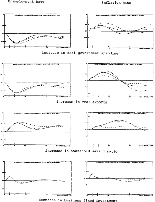
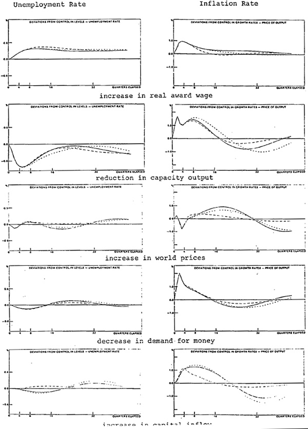
The unbroken lines represents the outcome with the estimated bond rate reaction function. As tables 1 and 2 and the relevant panels in the diagrams of Appendix D indicate, the use of this regime usually produces an outcome for the growth of money which is less variable than the case in which the bond rate is fixed (the short dashes) but more variable than the case of non-accommodating money (the long dashes).
Table 3 summarises the variation from the control solution values of unemployment and inflation for each regime for monetary policy. It does this by presenting measures of the standard deviation of the solution path for the first four years[13] for each impulse. The standard deviations are calculated relative to the control solution.
The general message from figure 2 and table 3 is simple. The variability of unemployment is reduced slightly by controlling the growth of money for three of the four disturbances to real demand and the shocks to capacity output, world prices and capital inflow. When the shock is an increase in minimum wages, controlling money makes the peak effect on unemployment slightly higher than it is when the impulse is accommodated. In the case of a reduction in money demand, the natural responses of the model are to reduce the money supply, and when the money stock is controlled so that the fall is offset by reductions in the bond rate the initial output performance is slightly stronger. As a result unemployment rises by less later in the period. In no case does the response of unemployment vary by much according to the regime for money policy. In RBA79, there is little which monetary policy can do to offset the real effects of the disturbances considered here. In some cases the effects on employment (and output) are sizeable, and the main question is perhaps whether monetary policy can prevent the shocks from occurring. This point is discussed below.
In contrast to unemployment, the longer-run response of inflation varies more obviously with different regimes for monetary policy. For all impulses, the amplitude of the cycles in inflation are reduced, in some cases substantially, when money is controlled. In the short-run, however, the direct effects of the shocks dominate the model's responses and in most cases a sizeable increase in prices results even when money is controlled.
| Unemployment Rate | Inflation Rate | |||||
|---|---|---|---|---|---|---|
| Rigid bond rate | Partially accommodating money | Tight money | Rigid bond rate | Partially accommodating money | Tight money | |
| Increase in gov't spending | .50 | .44 | .41 | .95 | .66 | .54 |
| Increase in exports | .52 | .48 | .41 | 1.11 | .95 | .62 |
| Increase in savings ratio | .39 | .38 | .44 | .60 | .60 | .33 |
| Decrease in investment | .15 | .15 | .13 | .31 | .31 | .28 |
| Increase in award wages | .27 | .26 | .30 | .60 | .60 | .55 |
| Decrease in capacity output | .50 | .47 | .46 | 1.32 | 1.16 | 1.10 |
| Increase in world prices | .07 | .07 | .06 | .42 | .52 | .36 |
| Decrease in money demand | .08 | .08 | .09 | .87 | .87 | .89 |
| Increase in capital inflow | .10 | .09 | .05 | 1.12 | 1.03 | .61 |
|
* The figures represent the standard deviation of the deviation from control, calculated around the origin. |
||||||
When the shock consists of a reduction in the demand for money, controlling the money stock means offsetting the natural tendency for money to be reduced, and prices are higher as a result. In the medium term,if the interest rate is fixed inflation is on average less, but more variable, than in the case when money is controlled.
3.4 Sensitivity analysis
RBA79 is a model in which money has an important role. Prices and wages are highly variable, with an important direct effect upon inflation of the excess demand for money. In this section the effect of making the model progressively more “Keynesian” is examined.[14] Specifically, the following changes to the model are considered:
- omitting the direct effect of excess money on inflation;
- assuming that wages are exogenous;
- assuming that wages and prices are exogenous.
To simplify the discussion only two shocks are considered – an increase in the saving ratio and a cut in money demand. The panels of figure 3 illustrate the effect of an increase in the saving ratio on inflation and unemployment. The first panel repeats from figure 2 the results from the complete model. In this case, only two regimes for monetary policy are considered – parially accommodating money and tight money.[15] The second panel summarises the results when excess money is omitted from the price equation. In this case, the rate of inflation falls as unemployment rises. This occurs with both regimes for monetary policy. This is because when the direct money supply effect is omitted from the price equation, the effect of depressed demand in the goods market dominates the response of prices. In this case, controlling money has little effect on inflation, since even with accommodating money the supply of money is approximately equal to its control solution value. (Some complex full system interactions produce this result; an important factor is that, when the shock reduces prices the non-bank take-up of bonds is greater and bank lending is lower. Consequently, the tendency for reduced imports to raise the supply of money is offset by smaller domestic credit expansion.)
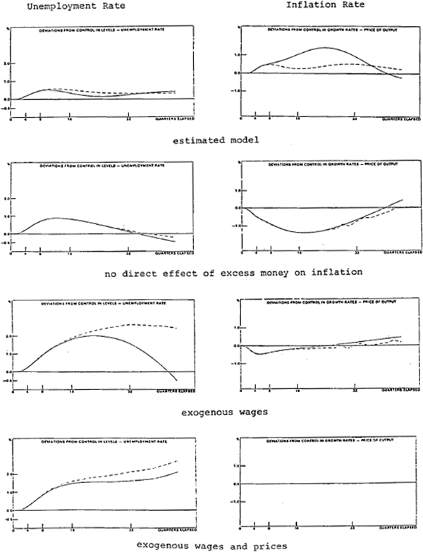
With wages exogenous and excess money excluded from the price equation, the tendency for inflation to fall below control is greatly moderated. (This is illustrated in the third panel of figure 3.) In this case the normal wage-price spiral is deleted, and the main influence on prices is the effect of lower demand for goods. Since prices fall while wages are fixed, unemployment increases by more than in the case in which both wages and prices fall, then falls as activity recovers and prices begin to increase.
When both wages and prices are fixed, as in the results of the fourth panel of figure 3, the fall in output is sustained for longer than it is with flexible prices and wages. As a result, unemployment continues to increase throughout the simulation period.
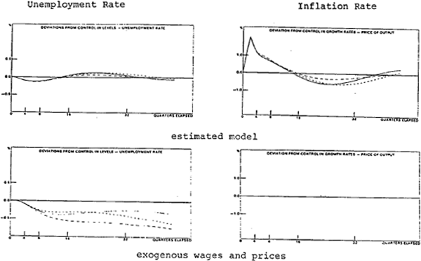
The panels of figure 4 show the results of a cut in money demand. The first panel again repeats from figure 2 the results with the complete model. The second panel has the results when prices and wages are exogenous (i.e. this corresponds to the fourth panel of figure 3). The main point to note from this comparison is that when prices are exogenous the results are more strongly in accord with Poole's (1970) analysis. That is, controlling money in the face of a change in the demand for money (the results are indicated by the long dashes) produces a path for output and employment which is considerably more variable, relative to the path with fixed interest rates (represented by the short dashes) than in the model with variable prices. This illustrates that when prices are allowed to vary they provide some offsets to the monetary effects of the disturbance. This is a similar result to that found for the increase in the saving ratio, and applies for most of the shocks considered in this paper.
3.5 Underwriting
As mentioned above, one of the main ways that tight monetary policies might improve the performance of the economy is by preventing shocks of the type considered in this paper. An example illustrates the potential importance of this point. This example uses the full model of the sections before the previous one.
The solid line in figure 5 shows the combined effect of two shocks – an increase in minimum wages followed 3 years later by a rise in the saving ratio. In each case the shocks are partially accommodated. Inflation expands and unemployment increases, in each case substantially. It will be recalled that in the earlier analysis of each of these shocks on its own, tight money moderated inflation in the medium term at the cost of a short-term rise in unemployment. At no time, however, did the different response of monetary policy make a great difference to the response of unemployment. In the simulation path represented by the dashed line in figure 5 it is assumed that tight money is maintained when the increase in wages occurs and that, as a result, a later rise in the household saving ratio does not occur. In this case, tight money produces a substantial medium-term benefit for both inflation and unemployment.

Footnotes
The dot represents the permanent (or steady state) effect of the shock. [9]
In the price equation of RBA79 the excess demand for money has a stronger influence than the excess demand for inventories, which represents the effect of demand pressure in the goods market. [10]
Which could be induced by a once-for-all reduction in productivity or by the effective loss of part of the capital stock. [11]
Evans (1979) provides an application for the case of an increase in government spending, for an earlier version of RBA79. [12]
The first four years are used for this comparison since most of the interesting action occurs in this period. The results for longer periods are similar. [13]
The type of dissection experiments considered here have been used to good effect by Helliwell and Higgins (1976) in analysing the RDX2 model. [14]
As in the earlier graphs, the results for partially accommodating money are indicated by the solid lines and the results for controlled money are represented by the dashed line. [15]