RDP 8502: Meeting on Monetary Issues II The Demand for Money in Australia: A Selective Survey and Some Updated Results[*]
November 1985
- Download the Paper 981KB
i Introduction
This survey was prepared for a conference on monetary matters held at the Reserve Bank of Australia in August 1985. The purpose of the paper was to shed some light on the hypothesis that reintermediation and increased intermediation had distorted the relationship between money, broadly defined, and its determinants.
The approach of the paper is straightforward. If reintermediation is, in fact, occurring then estimated money demand equations should tend to underpredict the actual growth of the relevant monetary aggregate. The results presented below found that this was indeed the case.
Rather than attempt to specify new demand for money functions, it seemed that it might be useful to examine the hypothesis by updating previously reported money demand studies. More than 20 such studies have been published over the past 15 years. The earlier studies were summarised by Davis and Lewis (1979). The past five or six years have seen a renewed burst of activity in this field with particular attention being paid to the stability of the demand for money in the 1970s. An updated version of the Davis and Lewis summary table is shown in the Attachment.
Almost all previous studies consider the demand for M1 or M3, although some consider particular components of these aggregates and a recent study by Drane et. al. (1985) considers some broader aggregates. Use of a variety of income and interest rate measures further complicates comparison, but some broad conclusions can be drawn from the published research. The long run income elasticity of money demand appears to be about one – few studies show a larger figure. Most studies successfully identify a long run “cross” interest rate elasticity whose value clusters around −0.4. The adjustment process appears to stretch to at least several quarters. There is little agreement on the question of the general stability of the money demand function.
Section ii presents some graphical evidence on movements in the key variables generally regarded as important in the analysis of money demand. Section iii considers some previously reported equations and updates them with a view to observing their behaviour over the past few years. (In selecting the equations to update, we have generally preferred wide rather than very narrow definitions of money. This reflects the view that since the regulatory changes of the early 1980s, M1 in particular is not a useful variable on which to focus.) Section iv reports some very preliminary work on the demand for broad money. Section v draws some conclusions.
ii The Statistics
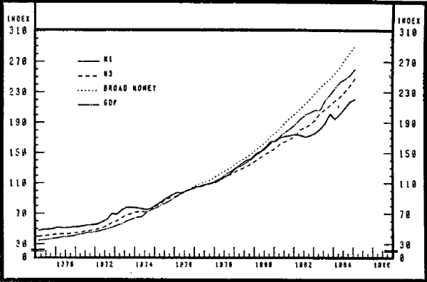
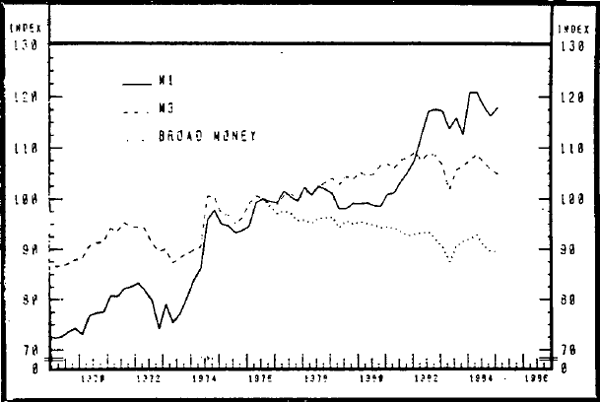
Graph 1 shows some data on M1, M3, and Gross Domestic Product (GDP) from 1969 to early 1985. Data on broad money are added from 1977. Between September 1977 and March 1985 GDP grew by around 160 per cent. Broad money grew more rapidly, by 190 per cent, while M3 grew by 150 per cent. Graph 2 shows the trends in velocity implicit in Graph 1. Over the period shown. M1 velocity has increased sharply, M3 velocity has risen more gradually, while the velocity of circulation of broad money has declined.
INDICES OF M1, M3, BROAD MONEY AND GDP
INDEX OF VELOCITY:
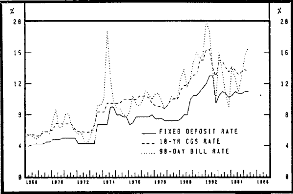
Many interest rates have been used in studies of the demand for money. Most studies use a government bond rate or the 90-day commercial bill rate as a cross rate. A smaller number of studies attempt to identify an own rate on money. Some indicative own and cross rates are shown on Graph 3. Those shown are the interest rate on trading bank fixed deposits, the interest rate on 10 year government bonds and the interest rate on 90 day commercial bills. While there is some general positive correlation between the rates, very significant differentials have opened up at various times. For instance in the June quarter of 1974 there was a 10 per cent differential between the bill rate and the other rates shown on Graph 3. This suggests that the choice of interest rate in money demand equations may be important.
INTEREST RATES
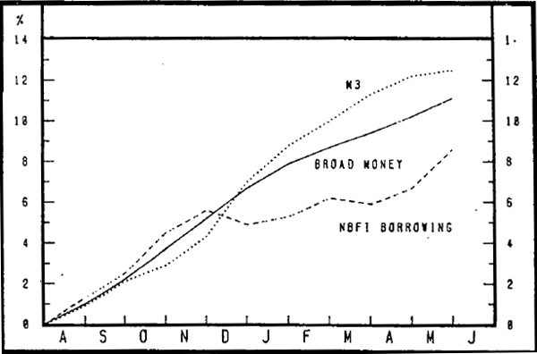
The long-run picture of the monetary aggregates stands in some contrast to developments over the past financial year. The long-run trend is one of more rapid growth in Non-Bank Financial Intermediary (NBFI) borrowings than growth in M3. The most recent year, however, has seen a period in which this picture has been reversed. Graph 4 shows cumulative percentage changes in M3, non-bank borrowings and broad money since July 1984.[1] The year can be conveniently divided into two (or three) periods. During the first few months of the year. M3 and NBFI borrowings grew more or less in line, although at the time there was some surprise that NBFI borrowings were growing more strongly following the 1 August measures. This may have reflected some jockeying for position by non-bank intermediaries. However, the following four or five months saw the situation change markedly. M3 grew rapidly, while there was little net change in NBFI borrowings between November and March. More recently, NBFI borrowings have again picked up, although cummulative growth of NBFI borrowings has been well below that of M3.
GROWTH IN MONETARY AGGREGATES
Over the year to June 1985, M3 grew by more than 17 per cent. Nominal GDP was growing by around 10 per cent and interest rates rose. As noted, existing econometric studies suggest an income elasticity of up to one and a negative interest elasticity. This conjunction of facts immediately suggests that conventional money demand functions are not likely to have been capable of explaining M3 growth in 1984/85 at all well.
iii Previous M3 Studies Updated
It is convenient to classify the Australian studies of the demand for money into three broad categories:[2]
- equilibrium studies assume that the demand for money adjusts completely within the current quarter (or year if annual data are used for estimation). There is no distinction between the long-run and short-run demand for money.
- disequilibrium partial adjustment models ate those most commonly employed in Australia and overseas. In these models a desired demand for money, Mt*, is combined with a lagged adjustment mechanism (usually the simple Koyck lag) to yield a predicted demand for money, Mt. Examples of this approach include Porter's (1979) technical paper for the Campbell Committee, Sharpe and Volker (1977), Freeland (1984) and Drane, Marzouk and Valentine (1985).
- whole system disequilibrium models in which money plays the role of a buffer stock. In models of this type, the parameters in the implicit money demand function are estimated indirectly in the equations in which monetary disequilibrium plays an important role. The Reserve Bank's RBII model is an example of this approach. In that model, monetary disequilibrium plays an important role in many equations including those for prices, consumption and the demand for bonds.
Identifying emerging shifts in econometric relationships is always difficult. Formal tests such as the Chow test or the QSUM test are unlikely to show statistically significant results if the shift is just beginning to occur. Most such tests require a reasonable run of data on both sides of a break in series before any rigorous conclusions can be drawn. However there are two informal, but suggestive, tests of the stability of the relationship being modelled. The first is to compare values of the estimated parameters when the relationship is estimated over differing sample periods. Any apparently sizeable difference in the estimates between the sample periods may be indicative of an alteration in the relationship between the dependent and independent variables. The second test is to compare the actual growth in the relevant monetary aggregate with that predicted by the equation. This may be the only way in which to identify the possibility of a very recent breakdown in a relationship. Setting standards by which to judge the significance of divergences in actual and predicted growth rates is of course subjective.
The following paragraphs examine the recent performance and predictive ability of previously estimated models, from each of these classes. In each case, the model is updated to the period for which a full data set is available. In the case of quarterly models, this is 1985(1) and for the one annual model considered, 1983/84. Reflecting the balance of the Australian literature, the bulk of models reported are disequilibrium partial adjustment models.
Partial Adjustment Disequilibrium Models
This section analyses four previous studies.
- Sharpe and Volker (1977):
- Porter (1979):
- Freeland (1984):
- Drane, Marzouk and Valentine (1985).
Sharpe and Volker
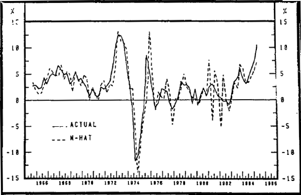
Taking up some earlier work by Juttner and Tuckwell (1974). Sharpe and Volker estimated several specifications of money demand functions using quarterly data for the period 1952(2) to 1972(3). For each specification two equations were estimated, one including the rate on two year government bonds and the other containing a long-term interest rate, the rate on ten year government bonds. The specification updated here is the conventional demand for money specification with real M3 balances depending on nominal gross national expenditure (deflated by the CPI) and interest rates. A simple Koyck lag structure was used. Table 2 compares the characteristics of the original Sharpe and Volker equation with the updated equation estimated using data for the period 1952(2) to 1985(1).[3]
| Variable | S1 (Short Rates) | L1 (Long Rates) | |||
|---|---|---|---|---|---|
| Original 1952(2)–1972(3) |
Updated 1952(2)–1985(1) |
Original 1952(2)–1972(3) |
Updated 1952(2)–1985(1) |
||
| Constant | .427 (2.60) |
.364 (3.56) |
.400 (2.52) |
.343 (3.70) |
|
| GNE | .225 (5.13) |
.193 (5.06) |
.192 (4.73) |
.155 (4.07) |
|
| CGS | −.056 (3.12) |
−.041 (2.80) |
−.095 (3.29) |
−.026 (1.68) |
|
| (M3/P)−1 | .756 (13.95) |
.774 (15.50) |
.797 (15.27) |
.807 (16.62) |
|
| R2 | .99 | .98 | .99 | .99 | |
| Implied Long Run Elasticity: | |||||
| GNE | .922 | .854 | .946 | .803 | |
| CGS | −.230 | −.181 | −.468 | −.135 | |
Where CGS = interest rate on two year Commonwealth Government securities.
Comparing the estimated parameters of the original and updated equations suggests little
structural change. Graph 5 plots the results from the first of these equations for growth in
M3, and M over the sample period.[4]
The graph includes estimates for the June quarter of 1985[5] which suggest that  grew
more rapidly in 1983/84 and much more slowly over the past year than M3.
REAL M3: SHARPE AND VOLKER STUDY:
Porter
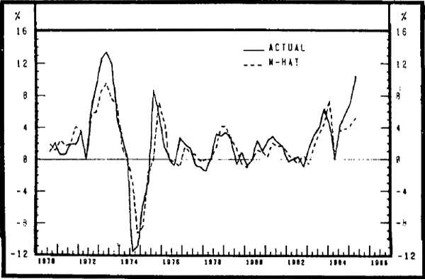
Porter reported conventional equations for M3, with slight variations in the estimation period. In general, these variations yield only slight differences to the estimated parameters. The equation chosen for comparison is that estimated over, the period 1966(3) to 1979(2). The new estimates are shown below in Table 3.
| Variable | Oriqinal 1966(3)–1979(2) |
Revised 1966(3)–1979(2) |
Updated 1969(3)–1985(1) |
|---|---|---|---|
| Constant | 1.46 (2.17) |
.636 (1.30) |
.016 (.03) |
| GDP | .204 (3.70) |
.218 (3.95) |
.249 (4.71) |
| CGS | −.073 (4.40) |
−.060 (3.60) |
−.056 (4.11) |
| (M3/P)t−1 | .818 (10.38) |
.747 (9.11) |
.774 (10.34) |
| R−2 | .976 | .959 | .950 |
| Durbin's h | .324 | .012 | .221 |
| Implied Long Run Elasticity: | |||
| GDP | 1.12 | 0.862 | 1.102 |
| CGS | −.401 | −.237 | −.247 |
Graph 6 shows the results from the updated Porter model. The results are similar to those obtained by updating the Sharpe and Volker model. Once again, there is evidence that the equation tended to overpredict M3 growth in 1983/84 and underpredicted growth in the second half of 1984/85.
REAL M3: PORTER STUDY:
Freeland
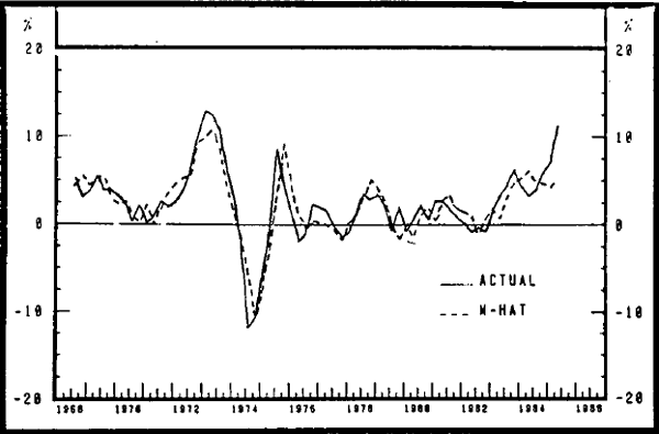
Freeland (1984) estimated a standard money demand function over the period 1967(3) – 1983(2). The statistical properties of the equation and the estimated coefficients were virtually unchanged when the equation was re-estimated with revised data over the original sample period and over the period 1967(3) to 1985(1). The results from the original equation and those from the longer sample period are reported in Table 4.
| Variable | Oriqinal 1967(3) – 1983(2) |
Updated 1967(3) – 1985(1) |
|---|---|---|
| Constant | 1.031 (2.85) |
.984 (2.95) |
| GDP | .229 (4.94) |
.226 (5.11) |
| CGS−1 | −.110 (6.08) |
−.113 (6.32) |
| RSSA−1 | .024 (2.91) |
.028 (3.45) |
| RFD−1 | .065 (2.91) |
.063 (2.86) |
| (M3/P)−1 | .693 (11.44) |
.703 (12.32) |
 |
0.98 | 0.98 |
| Durbin's h | .37 | .18 |
| Implied Long Run Elasticity: | ||
| GDP | 0.746 | 0.761 |
| CGS−1 | −.358 | −.380 |
| RSSA−1 | .078 | .094 |
| RFD−1 | .212 | .212 |
|
Where: RFD = Interest rate on trading bank fixed deposits. Comprises the rate on 18 to 24 month deposits to 1971(4). the rate on deposits of 24 months maturity from 1972(1) – 1974(2), and the mid-point of the range of 24 to 48 month deposits thereafter. RSSA = Interest rate on savings bank statement accounts. This comprises the minimum of the range on ordinary savings accounts under $4,000 up to December 1979, and the mid-point of the range on statement savings accounts thereafter. |
||
In general, the estimated parameters of both equations are plausible. The interest rate on two year government securities played the conventional role of the rate on competing assets in the money demand function; it has the expected sign and is highly significant. The interest rates on balances included in M2 and M3 were included as own rates of interest and, as expected, their signs were positive in both sets of results. The adjustment speeds for each equation were also similar; 2.25 and 2.37 for the original and updated version respectively. The long run income elasticity for each was approximately 0.75 – perhaps a little low compared with previous studies.
Graph 7 shows the results from the updated Freeland equation. On average, the equation appears to perform quite well. However, in the recent March and June quarters the equation clearly underpredicts, giving a pattern of errors seemingly out of character with the earlier results. This equation also suggests the relationship between M3 and the explanatory variables has shifted – M3 has been growing faster over the past year than can be explained by movements in the variables that have previously explained its demand.
REAL M3: FREELAND STUDY:
Drane, Marzouk and Valentine
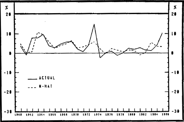
Using annual data from 1958/59 to 1982/83 Drane, Marzouk and Valentine estimated a series of equations for M1, M3 and two broader aggregates – one similar to broad money and a wider credit aggregate. The broader aggregates, MM and DCMM, are those previously developed by Marzouk and Drane (1983).
In contrast to the quarterly studies, Drane et. al. do not find a significant role for GDP in determining demand for M3. As an alternative, they use company gross operating surplus as a measure of transactions demand for money. However, it is shown below that when the time trend is omitted, GDP becomes significant so we have concentrated on the conventional specifications labelled (B.4) by Drane et. al. The results of re-estimation with the latest data and updating to 1983/84 are shown in Columns 2 and 3 of Table 5.
The above problems with the original equation remain when it is updated. In particular, the co-efficient on GDP remains insignificant. It seemed likely that there was co-linearity between the time trend and GDP which could explain the small coefficients and the large standard errors. This was confirmed when the equation was re-estimated omitting the time trend. These results are shown in Column 4 of Table 5. This seems a superior form on all counts.[6]
| Variable | (1) | (2) | (3) | (4) |
|---|---|---|---|---|
| Oriqinal (1958/59–1982/83) |
Revised (1958/59–(1982/83) |
Updated (1958/59–1983/84) |
Updated (1958/59–1983/84) (excl. time) |
|
| Constant | .23 (0.64) |
.352 (0.79) |
.337 (.83) |
−.125 (1.53) |
| GDP | .205 (1.17) |
.173 (0.72) |
.177 (0.78) |
.405 (3.47) |
| Interest Rate | −.132 (3.82) |
−.151 (4.34) |
−.150 (4.57) |
−.129 (4.72) |
| Time | .005 (1.11) |
.007 (1.08) |
.007 (1.16) |
– |
| (M3/P)t−1 | .736 (5.22) |
.747 (4.38) |
.747 (4.49) |
.627 (4.77) |
 |
.993 | .9912 | .9918 | .9917 |
| Durbin's h | .23 | 1.439 | 1.32 | 1.26 |
| Implied Long Run Elasticity | ||||
| GDP | .777 | .684 | .700 | 1.086 |
| Interest Rate | −.500 | −.597 | −.593 | −.346 |
The growth rates for  implied by the updated equation (including
the time trend) are shown in Graph 8. As with the quarterly equations examined above, this
shows underprediction of M3 growth in 1984/85. Once the role of GDP is more accurately
pinned down as in the equation shown in Column 4 of Table 5. the underprediction in 1984/85
is a little more marked than that shown in Graph 8.
REAL M3: DRANE ET. AL. STUDY:
Buffer Stock Disequilibrium Models
RBII
The quantity of money is not directly determined by demand in RBII. Rather, the demand for money is implicit and estimated indirectly by using monetary disequilibrium (M* – M) as an argument in several equations of the form:
M* is determined by income and a vector of interest rates. Thus equations including monetary disequilibrium are estimated in the form:
The values in the various equations in which money demand appears are constrained to be equal across equations. The model was estimated in continuous time using full information simultaneous estimation techniques. The most recent full model estimation was over the period 1959(3) to 1980(4).
That version of the model can be seen as reflecting the structure of the financial system before deregulation and the floating of the exchange rate. A decision was taken some time ago that, since many fundamental relationships in the financial sector had altered as a result of institutional and regulatory changes in the 1960s, re-estimation of the model with data that did not reflect these developments was not likely to be very fruitful. However, Fahrer and Rankin (1984) have reported some work in which they made some modifications to the estimated money demand equation to reflect the likely effects of deregulation. In particular, various parameters were imposed at values which reflect the fact that the demand for money may become less sensitive to all interest rates and that money demand was homogenous of degree zero in all interest rates (the own rate, and bond and bill rates taken together). Their resulting equation was:
Where:
| M* | = | desired real M3 balances |
| mo | = | a constant |
| y | = | real GDP |
| rm | = | interest rate on trading bank fixed deposits |
| rb | = | interest rate on ten year government bonds |
| rb1 | = | interest rate on 90 day commercial bills. |
Graph 9 shows growth in RBII's implied M* using this equation. Growth in M* is quite volatile, partly reflecting the imposed unitary income elasticity of money demand and the quarter to quarter volatility of movements in GDP but more importantly, quite significant shifts in interest rate differentials. Once again, it seems clear that money growth over recent years has been moving in directions different to those suggested by movements in the assumed money demand function.
REAL M3: RBII
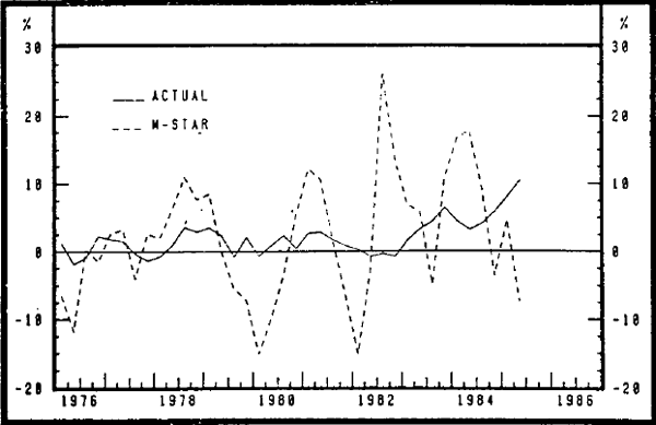
The results of this section suggests that M3 grew more slowly over 1983/84 and more rapidly over 1984/85 than can be explained by the updated versions of several money demand functions. It is interesting to note that when originally estimated parameters were used to generate predictions for growth over 1984/85, they tended to show even more marked underprediction. If recent strong growth in M3 simply reflects shifts in market share within the financial sector, equations for broader aggregates should suffer less from these problems. The following section turns briefly to this issue.
iv The Demand For Broad Money
The recent paper by Drane et. al. considered the demand for the aggregate MM previously developed by Marzouk and Drane. Rather than attempt to update MM, which was originally developed before the publication of the broad money aggregate, we have preferred to concentrate on broad money.[7]
As a first step, broad money was substituted for MM in the equation reported by Drane et. al. The results reported by Drane et. al. are shown as equation 6.1 in Table 6 and the results for broad money (using the same independent variable data set and deflation procedures as used by Drane et. al.) are shown as equation 6.2.[8] The results are broadly similar. The previous section showed the M3 equation to be better specified when time was dropped as an independent variable.
| Equation | Estimation Period to | Const. | GDP | Interest Rate | Time | Laqqed Dependent |  |
h | |
|---|---|---|---|---|---|---|---|---|---|
| 6.1 | MM Drane et.al Original data |
1982/83 |
.19 (.57) |
.337 (2.04) |
−.122 (3.49) |
.012 (2.56) |
.580 (3.99) |
.997 |
2.14 |
| 6.2 | Broad money, Drane et.al data | 1982/83 |
−.238 (.74) |
.444 (2.79) |
−.106 (3.12) |
.007 (1.82) |
.591 (4.31) |
.997 |
1.83 |
| 6.3 | Broad money Drane et.al, data, Excl. time | 1982/83 |
−.643 (2.67) |
.496 (3.01) |
−.082 (3.01) |
– |
.670 (4.89) |
.997 |
1.78 |
| 6.4 | Broad money Revised data | 1982/83 |
−.228 (.54) |
.445 (1.94) |
−.118 (3.16) |
.007 (1.33) |
.611 (3.46) |
.997 |
1.72 |
| 6.5 | Broad money Revised data Excl. time | 1982/83 |
−.647 (2.27) |
.556 (2.56) |
−.094 (2.82) |
– |
.621 (3.45) |
.997 |
1.70 |
| 6.6 | Broad money Revised data | 1983/84 |
−.268 (0.67) |
.451 (2.02) |
−.115 (3.21) |
.006 (1.34) |
.617 (3.58) |
.997 |
1.67 |
| 6.7 | Broad money Revised data Excl. time | 1983/84 |
−.659 (2.39) |
.563 (2.66) |
−.093 (2.87) |
– |
.616 (3.52) |
.997 |
1.69 |
The effect of dropping time from equation 6.2 is shown as equation 6.3 in Table 6. The explanatory power of the equation is not reduced and all co-efficients become significant.
When equation 6.2 was re-estimated using data incorporating the most recent revisions, the co-efficients obtained were similar to those reported by Drane et. al. but both time and GDP became insignificant. This result is shown as equation 6.4. When time was dropped from the equation (shown as equation 6.5) the co-efficient on GDP again became significant. Similar results were obtained when the equations were updated to 1983/84 (equations 6.6 and 6.7).
Graph 10 shows predictions based on equation 6.6 in Table 6.
REAL BROAD MONEY
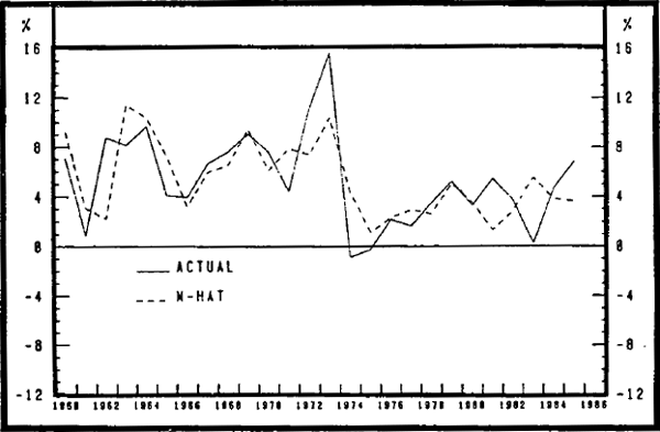
There was overprediction of  in 1983/84 and in 1984/85. (Similar
patterns of errors were found for equations 6.2, 6.3, 6.4, 6.5 and 6.7.)
Unfortunately, the results of these equations are ambiguous. While the finance company debenture rate (the rate used in equations 6.1 to 6.7) should have a negative coefficient for M1 or M3, in equations for MM or broad money, the sign of the debenture rate coefficient is a priori indeterminate. This is because the debenture rate is a cross rate for narrower components of the broad aggregate and an own rate for the broader components of the same aggregate. The sign of the coefficient will thus be a weighted average of these effects.
Some attempts have been made to overcome this problem, but at this stage, the results are not encouraging. An equation has been estimated with own and cross rates which have the appropriate signs, but the co-efficients on both interest rates are insignificant. Not surprisingly, the predictions of the equations are dominated by movements in GDP. They also show overprediction of broad money growth in 1983/84 and underprediction in 1984/85.
v Conclusion
The studies considered above suggest that with these specifications, estimated money balances tended to grow more rapidly than money supply over 1983/84 and grew significantly more slowly than money supply over the course of 1984/85. This largely reflects the fact that real GDP grew extremely rapidly over the course of 1983/84, but less rapidly in 1984/85. Nominal GDP grew by around 16 per cent over 1983/84 while M3 grew by around 11 per cent. In 1984/85 GDP grew at a more moderate pace, while monetary growth increased. Movements in interest rates, which were generally upward in 1984/85. provide no explanation within the conventional framework.
In both 1983/84 and 1984/85, it seems that additional factors must have been at work. One possible explanation for overprediction in 1983/84 is the use of actual rather than permanent income in estimating money demand functions. Strong predicted growth in M3 over 1983/84 appears to reflect the extraordinary bounce-back in economic activity following the drought and the recession. However in 1984/85, the major reason for underprediction appears to be that, especially since November 1984, banks appear to have been winning an increased share of intermediated business.
If the underprediction of equations for M3 in 1984/85 was solely due to reintermediation, it could be expected that broad money might have grown more in line with its traditional determinants over the past year than has M3. However, although equations for broad money remain poorly defined, it seems that broad money has also grown more rapidly than suggested by its previous determinants. This suggests the possibility of an increase in intermediation in 1984/85.
Footnotes
J.M. Veale, L.F. Boulton and W. Tease. [*]
July 1984 was chosen as a base as this was the first month some transactions between NBFIs could be identified. The data for broad money shown in the graph exclude this identified double-counting. [1]
The studies reported in this paper, excluding that for RBII, are standard partial adjustment models. There are no examples of demand for M3 studies which have an equilibrium specification. However, the paper by Porter and Adams (1976) reports estimates of such a model for M1. It would have been desirable to consider other classes of model such as the Hendry error correction specifications. However, such a specification has not, as yet, been applied in demand for M3 studies, although Pagan and Volket (1981) use such a specification in estimating the demand for M1. [2]
Data revisions made it impossible to reproduce the results of the original Sharpe and Volker specification exactly. This should be kept in mind when comparing estimates for this and other studies. Revisions to national accounts data, in particular, have been considerable. Both sets of equations have been corrected for first order autocorrelation. [3]
In Graph 5 (and subsequent graphs), results are presented showing four quarter ended
growth rates for two series, actual M3 and the predicted series,  .;
[4]
When this paper was prepared for the August conference June quarter 1985 national accounts data were not available. Accordingly, June quarter growth in real GDP was assumed to be 1 per cent. Results shown in Graphs 5 to 10 are based on this assumption. In the event, June quarter GDP growth was 2.8 per cent and GNE growth 2.2 per cent. Growth in earlier periods was revised downwards. [5]
Note that the long-run income and interest rate elasticities now conform more closely to “standard” results. [6]
The aggregate MM differs from broad money in that it also incorporates estimates of borrowings of some institutions not reporting under the Financial Corporations Act. However, its correlation with broad money is quite high. [7]
Drane et.al. used end June observations for MM and year average data for GDP, giving a single observation for each financial year. [8]


