RDP 8604: Leading Indexes – Do They? 4. Forecasting Activity Variables
May 1986
This section takes up the criticism that leading indexes may not be useful since (at best) they provide forecasts of coincident indexes of the business cycle while policy makers are more concerned with individual series. We evaluate the validity of this criticism by considering the ability of the two leading indexes to forecast individual activity series. Unfortunately, we are somewhat limited by the availability of series, since we require them to be on a monthly basis in order to get an accurate estimate of the leads and lags involved. The activity variables chosen are retail sales, motor vehicle registrations, the ANZ index of industrial production, total employment and the inverse of the unemployment rate. One would expect all these variables to move contemporaneously with the business cycle.[16]
A number of two variable VARs consisting of a leading index and an activity variable were estimated. Again because the activity variables (and leading indexes) were seasonally adjusted, no adjustment for seasonality was required when fitting the VARs, although some adjustments for trends were made by the inclusion of the appropriately ordered polynomial in time.[17] The characteristics of these estimated VARs are described below. A comparison is also provided, in which both leading indexes and an activity variable are included in a VAR to determine whether either index dominates the other in terms of its contribution to the forecast variance of the activity variable.
(a) Retail Sales and Motor Vehicle Registrations
The results for the leading indexes' ability to forecast these activity variables are fairly similar and thus reported together. In sum, neither leading index helps forecast either retail sales or motor vehicle registrations.[18] That is, any information embodied in the leading indexes which may be relevant to forecasting these variables, is dominated by the information embodied in the lags of the variables themselves. Retail sales is in fact almost perfectly correlated with its own lags, so that the addition of lags of the leading indexes to the equation does not significantly reduce the forecast error variance. Even though motor vehicle registrations was not highly correlated with its own lags, the leading indexes do not significantly reduce the forecast error variance.[19] This can be seen from Table 5 below, which displays the marginal significance levels for tests of Granger causality in the four VARs.
| Equation |
Explanatory Variables | Equation |
Explanatory Variables | ||
|---|---|---|---|---|---|
| Retail Sales | MILI | Rtails Sales | NILI | ||
| Retail Sales | – | .6472 | Retail Sales | – | .2903 |
| MILI | .0003 | – | NILI | .3827 | – |
| Registrations | MILI | Registrations | NILI | ||
| Registrations | .1890 | Registrations | – | .1658 | |
| MILI | .5877 | – | NILI | .3479 | – |
One cannot reject the null hypotheses that neither leading index Granger causes either activity variable, at even a 15 per cent level of significance. Although not presented here, the variance decompositions and impulse response functions are in agreement with this result that neither of the two leading indexes is useful in forecasting motor vehicle registrations or retail sales.[20]
(b) ANZ Production Index
The ANZ index is a monthly, seasonally adjusted index of industrial production; data are available back to September 1966. The VAR containing MI's leading index and the ANZ production index required six lags plus a quadratic trend component, while the one involving National's leading index required eight lags and a linear trend component. Table 6 contains the results for the Granger-causality tests in these two VARs.
| Equation | Explanatory Variables | Equation | Explanatory Variables | ||
|---|---|---|---|---|---|
| Production | MILI | Production | NILI | ||
| Production | – | .0001 | Production | – | .001.4 |
| MILA | .1038 | – | NILI | .9972 | – |
The significance levels in Table 6 clearly indicate that there is strong one way Granger-causality running from each leading index to the ANZ index. It appears that this may be slightly stronger in the case of MI's leading index. Therefore, the leading indexes may be useful with respect to forecasting future levels of production (as measured in the ANZ index).
The decompositions of the forecast variances for the production index in the two VARs are presented in Tables 7 and 8. In both cases, for horizons of nine months or more at least 25 per cent of the forecast variance is contributed by innovations in the leading indexes. For slightly longer horizons of thirteen months in the case of MI's leading index and seventeen months for NI's leading index, over 50 per cent of the forecast variance comes from the leading index. Both of these results confirm that the leading indexes help to forecast the production index. One may also compare the relative merits of the two indexes by considering the relative sizes of the forecast variances. tables 7 and 8 clearly indicate that the forecast variance is considerably lower when using MI's leading index than when NI's index is used. A measure of the lead time in the relationship between each index and the production index can be observed in the impulse response functions (for one standard error innovations in each leading index) presented in Figures 3 and 4. From Figure 3, it can be seen that the lead time for MI's leading index is quite small at about five months.[21] By comparison, Figure 4 indicates that NI's leading index leads the production index by about eleven months. It is also interesting to note that much larger movements are required in the NI index, than In the MI index, to generate a given movement in production.
| K | K-Step Forecast Variance |
Per Cent Due to Innovations in: | |
|---|---|---|---|
| MILI | Production | ||
| 0 | 2.69 | 1.3 | 98.7 |
| 1 | 2.94 | 1.2 | 98.8 |
| 2 | 3.25 | 1.8 | 98.2 |
| 3 | 3.42 | 1.8 | 98.2 |
| 4 | 3.62 | 1.7 | 98.3 |
| 5 | 3.81 | 4.9 | 95.1 |
| 6 | 4.05 | 10.0 | 90.0 |
| 7 | 4.38 | 16.5 | 83.5 |
| 8 | 4.74 | 22.8 | 77.2 |
| 9 | 5.17 | 29.3 | 71.7 |
| 10 | 5.72 | 36.1 | 73.9 |
| 11 | 6.36 | 42.3 | 57.7 |
| 12 | 7.03 | 47.6 | 52.4 |
| 18 | 10.50 | 62.5 | 37.5 |
| 24 | 11.80 | 63.7 | 36.3 |
| 30 | 12.05 | 63.3 | 36.7 |
| 36 | 12.87 | 65.6 | 34.4 |
| K | K-Step Forecast Variance |
Per Cent Due to Innovations in: | |
|---|---|---|---|
| MILI | Production | ||
| 0 | 3.04 | 0.2 | 99.8 |
| 1 | 3.55 | 0.2 | 99.8 |
| 2 | 4.20 | 1.4 | 98.6 |
| 3 | 4.88 | 3.2 | 96.8 |
| 4 | 5.80 | 5.4 | 94.6 |
| 5 | 6.60 | 7.2 | 92.8 |
| 6 | 7.72 | 11.0 | 89.0 |
| 7 | 8.84 | 16.0 | 84.0 |
| 8 | 10.13 | 21.5 | 78.5 |
| 9 | 11.45 | 26.1 | 73.9 |
| 10 | 12.86 | 30.5 | 69.5 |
| 11 | 14.34 | 34.7 | 65.3 |
| 12 | 15.87 | 38.5 | 61.5 |
| 18 | 24.57 | 53.1 | 46.9 |
| 24 | 29.88 | 57.7 | 42.3 |
| 30 | 31.79 | 57.9 | 42.1 |
| 36 | 32.41 | 57.1 | 42.9 |
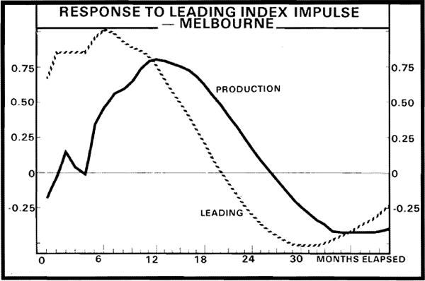
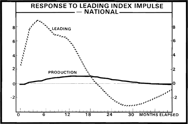
In terms of the informational lead times, these results indicate a two month informational lead time in the case of MI's index, and a six month informational lead for the NI's index.
(c) Employment and the Unemployment Rate
The final two activity variables we consider are employment and the inverse of the unemployment rate – it is inverted to obtain a procyclical variable.[22] Because the publication of these data has been on a monthly basis only since February 1978, the sample size used for the VARs containing these variables and the leading indexes is considerably smaller than previously. Before allowance is made for initial conditions, there are 80 observations compared with the 217 observations used for the previous three activity variables. Hence, the results using these employment variables should be viewed more cautiously.
In fitting these VARs only three or four lags and a linear trend were required to produce multivariate, white-noise residuals. Results for Granger-causal ordering tests for all four estimated VARs are presented in Table 9. These indicate that each leading index is useful in forecasting each employment related variable In the sense that each leading index significantly Granger-causes them. Further, there is evidence of feedback from each employment related variable into each leading index.
| Equation | Explanatory Variables | Equation | Explanatory Variables | ||
|---|---|---|---|---|---|
| Unemployment | MILI | Unemployment | NILI | ||
| Unemployment | – | .0005 | Unemployment | – | .0001 |
| MILI | .0001 | – | NILI | .0069 | – |
| Employment | MILI | Employment | NILI | ||
| Employment | – | .0001 | Employment | – | .0001 |
| MILI | .0005 | – | NILI | .0084 | – |
The variance decompositions for the forecast variance in the employment related variables are presented in Tables 10 through 13. They show the strength of the intertemporal causality from the leading indexes to the employment variables. In all cases, 50 per cent of the forecast variance in the employment variables comes from innovations in the leading indexes for horizons of one year and longer. With respect to both employment variables, the leading index published by the NI appears to yield a marginally lower forecast variance. This suggests that this leading index may provide more information on the future movements in employment than MI's index provides.
| K | K-Step Forecast Variance |
Per Cent Due to Innovations in: | |
|---|---|---|---|
| MILI | Unemployment | ||
| 0 | 0.14 | 1.9 | 98.1 |
| 1 | 0.24 | 2.5 | 97.5 |
| 2 | 0.31 | 3.0 | 97.0 |
| 3 | 0.39 | 5.1 | 94.9 |
| 4 | 0.46 | 8.8 | 91.2 |
| 5 | 0.53 | 13.2 | 86.8 |
| 6 | 0.61 | 18.0 | 82.0 |
| 7 | 0.68 | 23.1 | 76.9 |
| 8 | 0.75 | 28.4 | 71.6 |
| 9 | 0.83 | 33.6 | 66.4 |
| 10 | 0.90 | 38.5 | 61.5 |
| 11 | 0.97 | 43.0 | 57.0 |
| 12 | 1.04 | 47.0 | 53.0 |
| 18 | 1.47 | 58.4 | 41.6 |
| 24 | 1.81 | 53.8 | 46.2 |
| 30 | 2.05 | 48.3 | 51.7 |
| 36 | 2.26 | 49.9 | 50.1 |
| K | K-Step Forecast Variance |
Per Cent Due to Innovations in: | |
|---|---|---|---|
| MILI | Unemployment | ||
| 0 | 0.13 | 0.4 | 99.6 |
| 1 | 0.20 | 1.5 | 98.5 |
| 2 | 0.24 | 2.0 | 98.0 |
| 3 | 0.27 | 3.3 | 96.7 |
| 4 | 0.31 | 4.9 | 95.1 |
| 5 | 0.34 | 8.0 | 92.0 |
| 6 | 0.38 | 12.7 | 87.3 |
| 7 | 0.42 | 18.9 | 81.1 |
| 8 | 0.46 | 25.9 | 74.1 |
| 9 | 0.52 | 33.0 | 67.0 |
| 10 | 0.58 | 39.7 | 60.3 |
| 11 | 0.64 | 45.6 | 54.4 |
| 12 | 0.71 | 50.6 | 49.4 |
| 18 | 1.15 | 62.6 | 37.4 |
| 24 | 1.51 | 57.3 | 42.7 |
| 30 | 1.68 | 52.0 | 48.0 |
| 36 | 1.85 | 54.6 | 45.4 |
| K | K-Step Forecast Variance |
Per Cent Due to Innovations in: | |
|---|---|---|---|
| MILI | Employment | ||
| 0 | .035 | 0.7 | 99.3 |
| 1 | .049 | 0.9 | 99.1 |
| 2 | .064 | 0.7 | 99.3 |
| 3 | .077 | 1.8 | 98.2 |
| 4 | .091 | 4.9 | 95.1 |
| 5 | .105 | 9.5 | 90.5 |
| 6 | .119 | 15.3 | 84.7 |
| 7 | .135 | 21.9 | 78.1 |
| 8 | .152 | 28.9 | 71.1 |
| 9 | .171 | 35.8 | 64.2 |
| 10 | .191 | 42.3 | 57.7 |
| 11 | .212 | 48.1 | 51.9 |
| 12 | .235 | 53.1 | 46.9 |
| 18 | .375 | 66.8 | 33.2 |
| 24 | .469 | 63.5 | 36.5 |
| 30 | .513 | 58.8 | 41.2 |
| 36 | .560 | 60.4 | 39.6 |
| K | K-Step Forecast Variance |
Per Cent Due to Innovations in: | |
|---|---|---|---|
| MILI | Employment | ||
| 0 | .030 | 3.0 | 97.0 |
| 1 | .037 | 4.0 | 96.0 |
| 2 | .043 | 5.6 | 94.4 |
| 3 | .045 | 5.7 | 94.3 |
| 4 | .050 | 5.2 | 94.8 |
| 5 | .055 | 6.9 | 93.1 |
| 6 | .061 | 11.8 | 88.2 |
| 7 | .070 | 19.6 | 80.8 |
| 8 | .081 | 28.2 | 71.8 |
| 9 | .094 | 36.8 | 63.2 |
| 10 | .109 | 44.5 | 55.5 |
| 11 | .124 | 51.3 | 48.7 |
| 12 | .141 | 57.0 | 43.0 |
| 18 | .256 | 75.1 | 24.9 |
| 24 | .331 | 75.6 | 24.4 |
| 30 | .357 | 71.9 | 28.1 |
| 36 | .400 | 72.5 | 27.5 |
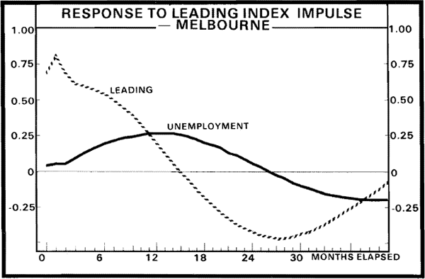
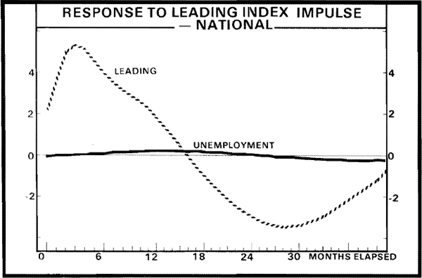
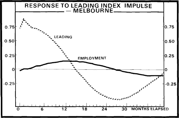
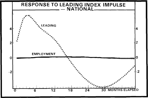
The impulse response functions (for one standard error impulses in the leading indexes) presented in Figures 5 through 8 indicate a lead time of approximately one year for each of the four VARs estimated. Thus, there is approximately a seven month informational lead time for the employment variables provided by the NI leading index, while the MI leading index yields a nine month informational lead time. Note again, however, that much larger movements in the NI index, than in the MI index, are required to induce a given movement in these employment variables.
(d) An Inter-Institute Comparison
We have demonstrated thus far that the leading indexes appear to be useful with respect to forecasting some activity variables that are coincident with the business cycle (the ANZ production index, employment and the unemployment rate inverted) and not very useful for others (motor vehicle registrations and retail sales). A comparison of the relative sizes of the forecast variance (in the activity variables) each index produced suggested that neither index was uniformly superior to the other. A more formal comparison of the two indexes may be obtained by nesting them in a composite VAR. This consists of both leading indexes and the relevant activity variable to determine which one dominates the other in terms of the Granger-causal ordering tests or the percentage contributions to the forecast variance of the activity variables.[23]
We only consider the three variable VARs for those activity variables that the leading indexes were found to be useful in forecasting – the ANZ production index, employment and the unemployment rate (inverted). For the ANZ production index eight lags and a quadratic trend component was required. The results of the Granger-causal ordering tests are provided below in Table 14.
| Equation | Explanatory Variable | ||
|---|---|---|---|
| Production | MILI | NILI | |
| Production | – | .0019 | .8023 |
| MILI | .9787 | – | .1180 |
| NILI | .2199 | .0023 | – |
Since we are most concerned with forecasting production, the figures in the first row are the most important. They clearly indicate that MI's index dominates NI's in terms of Granger-causing the ANZ index. Indeed, once the information contained in the lags of the production index and the MI leading index has been utilised, there is no role for the information contained in the lags of the NI leading index.
In considering the decomposition of the forecast variance of the production index into contributions made by innovations in the two leading indexes, we are faced with the problem of choosing which leading index contemporaneously causes the other.[24] To overcome this, we present the variance decompositions obtained under each of the two possibilities. These are presented in Table 15. In both cases MI' s leading index contributes a greater percentage of the forecast variance of production. Thus, on the basis of these results (and the earlier ones obtained from the two variable VARs), it would seem that MI' s index is superior to the NI index for forecasting industrial production.
| K | K-Step Forecast Variance |
Percent Due to innovations in: | ||||
|---|---|---|---|---|---|---|
| Orderinq 1 | Ordering 2 | |||||
| MILI | NILI | NILI | MILI | Production | ||
| 0 | 2.62 | 1.2 | 0.1 | 0.2 | 1.1 | 98.7 |
| 1 | 2.87 | 1.4 | 0.7 | 0.9 | 1.2 | 97.9 |
| 2 | 3.15 | 1.5 | 1.0 | 1.3 | 1.2 | 97.5 |
| 3 | 3.30 | 1.5 | 1.2 | 1.4 | 1.2 | 97.3 |
| 4 | 3.50 | 1.6 | 1.4 | 1.6 | 1.5 | 97.0 |
| 5 | 3.63 | 2.9 | 1.8 | 2.2 | 2.5 | 95.3 |
| 6 | 3.87 | 6.3 | 3.4 | 4.5 | 5.2 | 90.2 |
| 7 | 4.17 | 10.7 | 5.3 | 7.2 | 8.7 | 84.0 |
| 8 | 4.53 | 15.0 | 7.7 | 10.6 | 12.0 | 77.3 |
| 9 | 4.96 | 19.5 | 9.9 | 13.8 | 15.6 | 70.6 |
| 10 | 5.51 | 24.5 | 11.9 | 16.8 | 19.7 | 63.5 |
| 11 | 6.14 | 29.4 | 13.6 | 19.3 | 23.6 | 57.1 |
| 12 | 6.81 | 33.4 | 15.0 | 21.5 | 26.9 | 51.6 |
| 18 | 10.25 | 44.0 | 20.2 | 28.9 | 35.3 | 35.8 |
| 24 | 11.53 | 44.4 | 21.6 | 30.6 | 35.4 | 34.0 |
| 30 | 11.75 | 44.4 | 21.5 | 30.4 | 35.4 | 34.3 |
| 36 | 12.51 | 46.4 | 21.4 | 30.6 | 37.3 | 32.1 |
For the employment related variables both three variable VARs required four lags and a linear trend component. The results of Granger-causal ordering tests are presented for both models in Table 16 below.
| Equation | Explanatory Variable | ||
|---|---|---|---|
| Unemployment | MILI | NILI | |
| Unemployment | – | .7086 | .0652 |
| MILI | .0038 | – | .0131 |
| NILI | .1370 | .0201 | – |
| Employment | MILL | NILI | |
| Employment | – | .4017 | .0464 |
| MILI | .0096 | – | .0026 |
| NILI | .0559 | .2924 | – |
The figures in the first rows of the two sections of the table indicate the dominance of NI's leading index. However, this dominion is not as pronounced as the dominion by MI's index for the production index. The variance decompositions for the employment variables (again produced for both possible directions of contemporaneous causation between the leading indexes) presented in Tables 17 and 18 also show the dominance of NI's index. Innovations in the NI's index contribute a much higher percentage of the forecast variance for unemployment at all horizons than the contribution of MI's index. Again, this agrees with the earlier observation that the NI's index produced a lower forecast variance for this variable than did MI's index. However, for forecasting employment, the NI leading index only dominates the MI leading index at horizons longer than six months.
| K | K-Step Forecast Variance |
Percent Due to innovations in: | ||||
|---|---|---|---|---|---|---|
| Orderinq 1 | Ordering 2 | |||||
| MILI | NILI | NILI | MILI | Unemployment | ||
| 0 | .125 | 0.2 | 0.6 | 0.4 | 0.3 | 99.3 |
| 1 | .191 | 0.2 | 2.5 | 2.2 | 0.5 | 97.3 |
| 2 | .234 | 0.6 | 3.7 | 3.0 | 1.4 | 95.6 |
| 3 | .267 | 0.6 | 5.6 | 4.7 | 1.6 | 93.7 |
| 4 | .299 | 0.6 | 7.9 | 7.0 | 1.5 | 91.6 |
| 5 | .334 | 0.5 | 11.4 | 10.5 | 1.4 | 88.1 |
| 6 | .370 | 0.5 | 16.0 | 15.1 | 1.4 | 83.5 |
| 7 | .410 | 0.5 | 21.7 | 20.9 | 1.4 | 77.8 |
| 8 | .453 | 0.7 | 27.7 | 27.1 | 1.3 | 71.6 |
| 9 | .499 | 1.1 | 33.4 | 33.3 | 1.1 | 65.5 |
| 10 | .545 | 1.6 | 38.3 | 38.9 | 1.1 | 60.0 |
| 11 | .591 | 2.4 | 42.3 | 43.6 | 1.1 | 55.3 |
| 12 | .638 | 3.2 | 45.3 | 47.3 | 1.2 | 51.5 |
| 18 | .933 | 9.2 | 47.0 | 52.4 | 3.8 | 43.8 |
| 24 | 1.228 | 12.0 | 37.6 | 42.9 | 6.6 | 50.5 |
| 30 | 1.456 | 11.2 | 34.5 | 38.4 | 7.3 | 54.3 |
| 36 | 1.642 | 10.3 | 39.5 | 43.1 | 6.6 | 50.3 |
| K | K-Step Forecast Variance |
Percent Due to innovations in: | ||||
|---|---|---|---|---|---|---|
| Orderinq 1 | Ordering 2 | |||||
| MILI | NILI | NILI | MILI | Employment | ||
| 0 | .028 | 6.7 | 1.7 | 3.5 | 4.9 | 91.6 |
| 1 | .034 | 8.8 | 3.1 | 5.7 | 6.1 | 88.1 |
| 2 | .040 | 12.5 | 3.8 | 7.4 | 8.9 | 83.7 |
| 3 | .045 | 17.5 | 3.6 | 7.7 | 13.4 | 78.9 |
| 4 | .051 | 17.4 | 3.3 | 6.9 | 13.8 | 79.3 |
| 5 | .054 | 16.3 | 5.0 | 8.2 | 13.1 | 78.7 |
| 6 | .059 | 15.2 | 9.0 | 12.0 | 12.1 | 75.9 |
| 7 | .065 | 13.8 | 14.9 | 17.6 | 11.1 | 71.3 |
| 8 | .073 | 12.5 | 21.2 | 23.8 | 10.0 | 66.3 |
| 9 | .082 | 11.7 | 28.0 | 30.9 | 8.8 | 66.3 |
| 10 | .092 | 11.7 | 34.2 | 37.9 | 8.0 | 54.1 |
| 11 | .104 | 12.1 | 39.7 | 44.4 | 7.4 | 48.2 |
| 12 | .117 | 12.9 | 44.1 | 49.9 | 7.1 | 43.0 |
| 18 | .210 | 20.2 | 54.7 | 66.0 | 8.9 | 25.1 |
| 24 | .282 | 24.9 | 51.4 | 64.4 | 11.9 | 23.7 |
| 30 | .311 | 25.2 | 47.5 | 59.7 | 13.0 | 27.3 |
| 36 | .345 | 23.5 | 50.0 | 61.5 | 11.9 | 26.6 |
Footnotes
Boehm and Moore (1984) identify all these variables as ones that move with the cycle. Variable definitions and data sources are listed in the Appendix B. Appendix A contains the results of an analysis of the ability of the leading indexes to forecast quarterly GDP. These results, however, need to be interpreted with care because of the intertemporal smoothing involved in moving from the monthly leading indexes to quarterly series. [16]
A second order, or lower, polynomial. [17]
All four VARs required nine lags and a quadratic in time and were estimated over the period September 1966 to September 1984. [18]
In fact the equation explaining motor vehicle registrations was quite poor with an R2 of 0.7 as compared to the R2's of approximately 1.0 obtained for all other equations in this study. [19]
A possible reason for the inability of the leading indexes to forecast retail sales could be due to the fact that only a nominal retail sales series is available; movements in inflation could be masking the cyclical behaviour of real retail sales. [20]
Although it is slightly difficult to judge in the case of the first peak, since the leading index reaches a small turning point before turning completely at about six months after the impulse. The turning point at the trough is better defined. [21]
Note that we have scaled these variables. Employment is in units of one hundred thousand while the inverse of the unemployment rate has been multiplied by one hundred. [22]
These results should, however, be viewed with some caution. These tests may lack power due to multicollinearity of the two leading indexes. [23]
This problem did not occur previously because of the natural assumption that the leading index was contemporaneously exogenous to the activity variable. [24]