RDP 8802: Var Forecasting Models of the Australian Economy: A Preliminary Analysis 4. Forecast Evaluation
January 1988
- Download the Paper 787KB
The most obvious method of evaluating these forecasting models is to compare their ex-ante predictions with the actual outcomes. Benchmarks for this comparison can be provided by forecasts from other sources, preferably forecasts made on the basis of the same information as the models under scrutiny. Presumably, if a particular model performs better than alternative forecasts in ex-ante situations, then there is an a priori case that it may continue to do so in the future.
For this reason, we compare ex-ante forecasts from the three VAR models with nearly equivalent (publicly available) forecasts made by private and public sector organisations, as well as with the actual outcomes as per the June 1987 Quarterly Estimates of the National Accounts. The VARs are used to produce forecasts on the basis of data available at the time of the release of the December 1985 Quarterly Estimates of the National Accounts. The private sector forecasts are those obtained from surveys of private sector economists conducted by Business Review Weekly (Ries, 1986) and The Age (McCrann, 1986) and those provided by the Institute of Applied Economic and Social Research (Dixon and McDonald, 1986); public sector forecasts are taken from the Budget papers.
(a) Private Sector Forecasts
The Age, published a survey for calendar 1986 in January 1986.[10] Economists from thirty-six organisations were asked for forecasts of twenty domestic and international economic variables. Eight of these variables are contained in our VARs. Table 1 shows the actual outcomes for calendar 1986 (as per the June 1987 Quarterly Estimates), the average from The Age survey and unadjusted ex-ante forecasts from the VAR models. The figures in brackets give the proportions of individual forecasters who performed no better than the VAR models. An asterisk indicates that the survey average performed no-better than the VAR model.
| Variable | Actual | Survey | VAR(T) | VAR(D) | BVAR |
|---|---|---|---|---|---|
| GDPNF | 1.7 | 3.1 | 5.7(0) | 3.1*(16/35) | 7.5(0) |
| Prvte Invest. | −4.4 | 2.5 | 34.2(0) | 3.8(15/35) | 2.5*(22/35) |
| Unemployment | 629.7 | 616.7 | 671.2(13/35) | 661.9(19/35) | 673.8(11/35) |
| Current Acct. | 14.5 | 10.1 | 20.0(5/36) | 19.6(7/36) | 18.9*(25/36) |
| AWE | 7.1 | 7.8 | 9.7(1/35) | 11.8(0) | 6.5*(24/35) |
| CPI | 9.8 | 7.6 | 10.7*(34/36) | 8.4*(30/36) | 5.8(0) |
| TWI | 54.3 | 61.5 | 54.9*(35/36) | 59.4*(30/36) | 54.1*(36/36) |
| Bill Rate | 15.1 | 14.3 | 29.8(0) | 26.8(0) | 19.7(0) |
|
Note: The variables are defined as follows: |
|||||
Given the mechanical way we have constructed these VARs, and the large number (15) of variables in the models, their ex-ante forecasting performance rates reasonably well against the economists surveyed by The Age. VAR(T), which incorporates time trends, is relatively unimpressive. The remaining two VARs, which incorporate unit-root-like detrending, perform no-worse than a sizeable proportion of the survey respondents on most variables. The survey average is no better than VAR(D) for three of the eight variables, and no better than Figures in brackets give the proportions of individual forecasters who performed no-better than the VAR models. An asterisk denotes that the survey average performed no-better than the VAR model.
BVAR for four of the eight variables. What is particularly evident from the last two columns of Table 1 is that when the VARs miss the mark, they do so fairly significantly. This suggests that more attention to the trends or priors on certain individual variables may be particularly rewarding in terms of forecast accuracy.
Business Review Weekly (BRW) surveys eight economists each quarter. Forecasts in this survey cover changes in some sixteen economic variables for the next financial year. For example, forecasts published in April 1986 (drawing on information from the December 1985 Quarterly Estimates), forecast the financial year 1986–87.
As a result the forecasts generated with the VARs need to be compared with the BRW survey published in April 1986, when essentially the same information base was available to the economists as was used in generating the VAR forecasts. (The private sector economists did have the advantage of some additional monthly information.) Table 2 sets out the survey average of the BRW forecasts against the seven comparable forecasts from the VAR models. As for Table 1, an asterisk indicates that survey average performed no better than the VAR model, and the figures in brackets give the proportion of individual forecasts who performed no better.
| Variable | Actual | Survey | VAR(T) | VAR(D) | BVAR |
|---|---|---|---|---|---|
| GDPNF | 1.9 | 2.8 | 3.4 (0/8) | 1.8*(8/8) | 8.7 (0/8) |
| Prvte Cons | 0.5 | 2.2 | 1.9*(8/8) | 1.6*(7/8) | 4.9 (0/8) |
| Prvte Invest | −2.7 | 3.2 | 31.9 (0/8) | −1.3*(8/8) | 5.9 (1/8) |
| Imports | −4.7 | 3.4 | 4.7 (2/8) | 8.2 (0/8) | 8.7 (0/8) |
| Exports | 8.0 | 11.0 | 6.5*(8/8) | 8.0*(8/8) | 8.4*(8/8) |
| AWE | 5.7 | 7.8 | 7.5*(6/8) | 10.5 (0/8) | 3.7*(6/8) |
| CPI | 9.3 | 6.7 | 17.1 (0/8) | 8.6*(8/8) | 3.6 (0/8) |
Note: The first five variables are measured as 1986–87 on 1985–86 percentage changes; the last two are expressed as June quarter 1987 on June quarter 1986 percentage changes. |
|||||
The comparison with BRW survey forecasts shows the VAR forecasts performing at least as well or better on most variables. Model VAR(D) forecasts better than survey average for five out of seven variables, VAR(T) forecasts better for three out of eight; BVAR shows the least accuracy of the VAR models.
A similar result emerges when the VAR forecasts are compared with those from the Institute of Applied Economic and Social Research (IAESR) in Melbourne, which publishes forecasts periodically in The Australian Economic Review. The forecasts published by Dixon and McDonald (1986), for financial year 1986–87, are compared with the VAR forecasts in Table 3.
| Variable | Actual | IAESR | VAR(T) | VAR(D) | BVAR |
|---|---|---|---|---|---|
| GDPNF | 1.9 | 3.2 | 3.4 | 1.8* | 8.7 |
| Prvte Cons. | 0.5 | 1.7 | 1.9 | 1.6* | 4.9 |
| Prvte Invest. | −2.7 | −1.1 | 31.9 | −1.3* | 5.9 |
| Imports | −4.7 | −3.0 | 4.7 | 8.2 | 8.7 |
| Exports | 8.0 | 4.0 | 6.5* | 8.0* | 8.4* |
| Employment | 2.0 | 2.7 | 3.6 | 0.7 | 4.1 |
Note: The first five variables are measured as 1986–87 on 1985–86
percentage changes; the last is expressed as June quarter 1987 on June quarter 1986
percentage change. |
|||||
VAR(D) forecasts are better than the IAESR for four of the six variables reported here. The other two models appear much weaker, posting a better performance for one variable only.
Tables 1–3 provide evidence for the reasonable performance of VAR models against private sector forecasters. The most accurate forecasts are generated by the two VAR models which employ unit-root type detrending; larger errors appear when models are dominated by inappropriate detrending processes.
(b) Public Sector Forecasts
Each year some selective forecasts are presented with the Budget papers. Table 4 sets out forecasts from the 1986–87 Budget for the nine comparable variables.
| Variable | Actual | Budget | VAR(T) | VAR(D) | BVAR |
|---|---|---|---|---|---|
| GDPNFb | 1.9 | 2.5 | 3.4 | 1.8* | 8.7 |
| Prvte Consb | 0.5 | 1.25 | 1.9 | 1.6 | 4.9 |
| Importsb | −2.7 | −6.5 | 4.6 | 8.2 | 8.7 |
| Exportsb | 8.0 | 2.5 | 6.5* | 8.0* | 8.4* |
| Current Accountc | 13.5 | 14.6 | 23.0 | 21.2 | 21.3 |
| Employmentb | 2.0 | 1.75 | 3.6 | 0.7 | 4.1 |
| AWEb | 5.7 | 6.0 | 7.5 | 10.5 | 3.7 |
| CPIb | 9.3 | 8.0 | 17.1 | 8.6* | 3.6 |
| TWIa | 53.6 | 52.0 | 53.5* | 58.3 | 53.2* |
Note; |
|||||
VAR(D) and VAR(T) produce more accurate forecasts for two of the nine variables listed in Table 4 so that although the Budget forecasts are closer to “actual” on the whole, they do not completely dominate the naively generated forecasts.
(c) Actual Outcomes
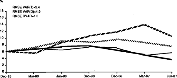
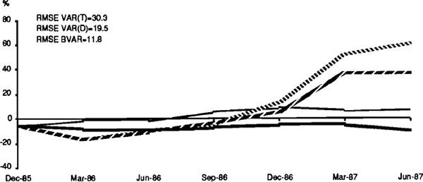
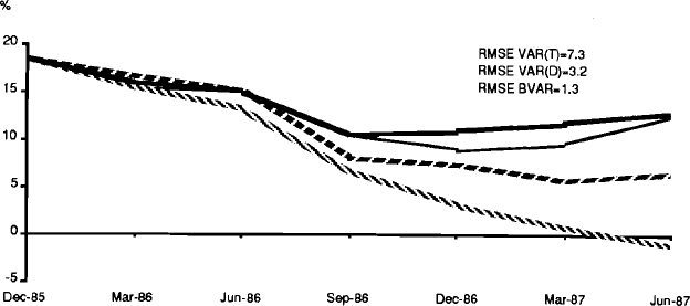
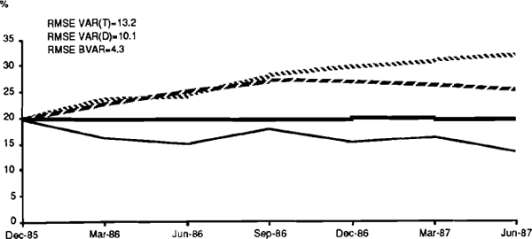
A final assessment of the forecasts is to graph the ex-ante predictions of the VAR models quarter by quarter to see how well they track the actual outcomes of each variable. Graphs of the variables, generally in twelve month ended percentage changes with root mean square errors for the period March 1986 through June 1987, are shown in Figures 1 through 15. (Any difference between the model and actual values in December 1985 are due to revisions in the data since early 1986).


The BVAR model is the best predictor for ten out of the fifteen variables. These results confirm Litterman's hypothesis that VAR's with Bayesian priors perform better than unrestricted models, all other things being equal.
However, all of the models have limitations as forecasting models. They appear to have been poor predictors of the turning points in some of the series, especially exports, imports and the current account balance. The end of 1985 marked a significant change in economic conditions. The general slowdown is evident in the downturn in GDPNF, consumption, investment and imports; a high proportion of the variables have turning points around the first quarter of 1986. The period for December 1985 to June 1987 provides a fairly stringent test of the VAR model's forecasting ability since most variables are not moving in line with earlier trends. The VAR(T) model in particular tends to move very strongly on trend and thus tends to perform badly over this period. The BVAR model is much less dominated by trend and consequently tracks the actual outcomes more closely.
Footnote
The economists surveyed by the The Age would not have had the benefits of the information in the December 1985 Quarterly Estimates. However, they did have current information on most of the variables. Any bias is likely to be offset by our use of the survey average. [10]