RDP 8813: The Fiscal Deficit and the Current Account: Twins or Distant Relatives? 2. Determinants of the Current Account Balance.
December 1988
- Download the Paper 816KB
In order to evaluate the effects of changes in fiscal policy on a country's external payments position it is necessary to make use of some model of current account determination. Simplifying assumptions need to be introduced to make the analysis tractable. Traditionally it has been common to apply what might be called an elasticities or trade-balance approach in view of the fact that a major component of the current account balance is the difference between the value of imports and the value of exports of goods and services. As a consequence the focus of attention has been on movements in some measure of the real exchange rate and in income by analogy with relative-price and income effects in consumer demand theory. From a theoretical point of view, the problem with this approach is that it proceeds as if the underlying reason for exchange rate changes did not matter for the trade balance, and as if income growth brought about by an exogenous expansion of demand had the same effect as that caused by an increase in supply. Empirically one might therefore have difficulties in isolating stable relationships between the current account and exchange-rate and income changes.
Partly in reaction to these difficulties with the elasticities approach, an alternative has recently been proposed that focuses on the economy's savings-investment balance. Since the current account is by necessity equal to the aggregate net savings of the economy, the proponents of this approach argue that it draws attention to those factors that have the most direct influence. In particular, variations in the real rate of interest and differences between current and expected future income are likely to influence significantly both the savings behaviour of households and the investment decisions by firms. Government fiscal policies such as changes in personal income and corporate taxes are also likely to be important in this context. The relationship between these policies and the current account seems more apparent viewed from this approach than from the elasticities approach.[2] This is all the more so since net savings of the economy as a whole is equal to the sum of the private sector's excess of savings over investment and the public sector's budget surplus.
While the savings-investment approach does steer attention in the appropriate direction by emphasizing the intertemporal nature of current account imbalances, it should be recognized that it too must be imbedded in a more complete model before conclusions can be drawn about the effects of exogenous shocks in general and about fiscal policies in particular. Such a model would not only have to take into consideration possible offsets between changes in the public sector's fiscal balance and the private sector's net savings, it would also have to account for indirect influences operating through changes in income, interest rates, exchange rates, etc.. These indirect effects are indeed exactly those that make sure that the elasticities and savings-investment approaches ultimately must give the same answer. In this sense then, they should be regarded as complementary rather than competing explanations of current account imbalances and as providing a check on the consistency of partial equilibrium arguments.
(a) A Minimal Formal Model.
With the aim to incorporate both the direct and the indirect effects of various disturbances and therefore to ensure consistency between the elasticities and the savings-investment approaches, the remainder of this section will use a small theoretical macro-economic model to investigate the link between various types of fiscal policies and the current account. To keep the analysis as transparent as possible the model abstracts from the longer-run feedback effects of debt (domestic as well as foreign) and capital accumulation. In addition, the functions describing the behaviour of economic agents are not explicitly derived from dynamic maximization problems facing households and firms. This will not have important consequences for the main points that are derived provided that care is taken in interpreting the policy shocks we are considering.[3]
The model consists of equations (1) – (9).[4] As it is essentially a variant of mainstream open economy models in the Mundell-Fleming tradition, only certain features will receive explicit comments.
Equation (1) equates the supply of domestic output with the demand for domestic output. Demand is in turn expressed in terms of its consumption, investment, government spending and net export components all expressed in terms of domestic output units. The only noteworthy aspect of that equation is the presence of the import tariff rate, tim which influences the internal relative price between the import good and the export good.
The definition of disposable income reflects the assumption that labour income, αy, is taxed at a rate t1, whereas income from capital, (1-α)y, is taxed at tk. Furthermore, interest earnings on holdings of net foreign assets and domestic government debt is not taken into account.
Domestic consumption is a function of disposable income and a tax parameter ts that is introduced to capture the effects of a tax on savings. This tax is assumed to be levied on that part of disposable income that is not consumed. While this may not be the manner in which incentives to save are most often influenced by tax policy, it is maintained here for reasons of analytical simplicity.[5] Similarly investment is assumed to depend on income accrued to capital, the real rate of interest and the tax rate on income from capital.
| y | supply of the domestic good |
|---|---|
 |
full-employment output of the domestic good |
| ydisp | disposable income |
| c | private sector aggregate consumption |
| i | private sector aggregate investment |
| gd (gim) | government consumption of the domestic (import) good. g = gd + gim |
| x | exports |
| im | imports |
| a (a*) | domestic (foreign) private sector absorption (= c + i) |
| π(πe) | corporate (expected) profits |
| r (r*) | the domestic (foreign) real rate of interest |
| e | the real exchange rate = the price of the import good in terms of the domestic good |
 |
the long-run value of e |
| P (P*) | the nominal price of the domestic (import) good |
| E | the nominal exchange rate |
| L | the real demand for money |
| M | the nominal money supply |
| α | labour share in total income |
| tk | tax rate on capital |
| t1 | tax rate on labour |
| tim | tax rate on imports |
| ts | tax rate on saving |
d, s, q are parameters of the system. |
|
Export demand depends on the external relative price, e, and on foreign absorption whereas import demand is a function of the internal relative price, domestic absorption, and government imports.
In equation (7) the real money supply is shown to depend on the domestic price level which reflects both the price of domestic output and the price of imports weighted by their respective share in domestic consumption. The money demand specification is traditional.
Within the period covered by the analysis the price of domestic output is assumed to adjust partially in response to deviations between actual output and a fixed level of full-employment output as in (8).[6]
Interest parity is assumed to hold. It is written in terms of real interest rates in (9) where
the term q ( – e) is assumed to capture the expected rate of
real depreciation of the domestic currency. Finally, for the sake of analytical simplicity it is
assumed that the nominal and real interest rates are equal.
The model can be reduced to a pair of equations reflecting goods market equilibrium on the one hand (equations (1)–(6) and (9)) and money market equilibrium on the other (equations (7)–(9)). These are drawn as the IS and LM curves respectively in Figure 1. The IS curve is upward-sloping since a real depreciation of the home currency (an increase in e) increases the demand for the domestic good and has to be accompanied by an increase in output for goods-market equilibrium to be maintained. In the money market, an increase in e increases the domestic price level and reduces the real supply of money. Output must fall to maintain equilibrium, so the LM curve is downward sloping.[7] The location of the curves depends on the values of the exogenous variables in the model, notably the supply of money and the level and composition of government spending as well as on the values of the various tax parameters. In the following implicit equations for the IS and LM curves respectively, displacements to the right are indicated by a (+) and those to the left by a (−) directly above the corresponding exogenous variable or parameter.
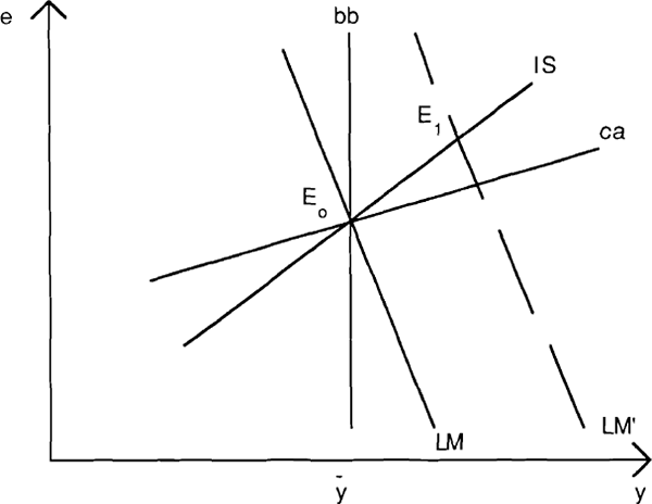
Two additional schedules are drawn in the figure. The curve labeled ca represents combinations of e and y that yield current-account balance. It is upward-sloping since a depreciation improves the trade balance and an increase in y deteriorates it. It will be flatter than the IS curve provided that the elasticity of the trade balance with respect to the real exchange rate is sufficiently large. Points lying above ca represent states of current account surplus and those lying below represent deficits. The bb line represents situations of public sector budget balance.
To a first approximation[8] the exchange rate effects on the expenditure and revenue side will cancel so that this line will be vertical. To the left of bb the budget is in deficit and to the right it is in surplus. The direction of displacements of the curves can be deduced from the following representations.
The intuition behind the signs is straightforward. For instance, an increase in government imports deteriorates the trade balance requiring a decrease in domestic income (which reduces private-sector imports) in order to maintain equilibrium. Increases in taxes on income reduce disposable income which in turn decreases imports. Current account balance can therefore be sustained at a higher level of income. In other words, increases in t1 and tk shift the ca schedule to the right.
The balanced-budget schedule shifts rightwards with increases in expenditures since the higher level of income is required to generate the extra revenues needed to maintain fiscal balance. For analogous reasons, increases in tax rates will shift the bb schedule to the left.
Before we proceed to a detailed analysis of the relationship between fiscal policies and the current account, it is instructive to consider the effects of movements in other variables, notably a change in monetary policy and exogenous changes in domestic and export demand. The consequences of these disturbances will be established using the graphical apparatus in Figure 1 in the hope that this will provide a better intuitive understanding of the adjustment mechanisms involved than a purely algebraic treatment.
The case of a domestic monetary expansion is by a shift of the LM curve to LM' in Figure 1. Starting from an initial equilibrium at E0 characterized by fiscal and current account balance as well as by full employment[9], the expansion will result in an increase in output and a currency depreciation at E1. The current account improves as does the public sector's fiscal balance. Both improvements can be seen as a consequence of the expansion of output resulting from the easier monetary policy. As output expands, the private sector will increase its savings making room for an improved external balance.[10] The fiscal balance improves as expanded economic activity increases tax revenues.
An increase in private sector autonomous spending is depicted in Figure 2 as a shift of the equilibrium from E0 to E1 implying an expansion of output and a currency appreciation. As before, the public sector fiscal balance improves because of increased tax revenues. Because part of the increase in demand is imported the current account schedule shifts to ca1. The new equilibrium is thus characterized by a significant current account deterioration. This deterioration is a direct consequence of the increase in domestic spending crowding out net exports.[11]
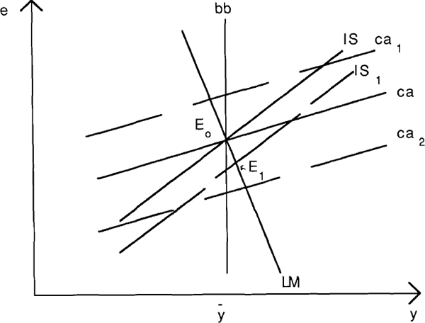
Comparing the responses of the current account and the public sector's fiscal balance to the shocks it is worth noting that the relationship between them is different in each of the two cases just considered. Whereas the fiscal balance improves in both examples, the current account deteriorates in one and improves in the other. This is an example of the general point that the relationship between any two endogenous economic variables is likely to depend on the type of disturbance that has occurred. As we shall have occasion to point out again, it is extremely important to keep this in mind when we attempt to account for actual historical variations in the current account and the fiscal balance.
An expansion of export demand is again illustrated in Figure 2 by a shift in IS to IS1. As before, the economy's new equilibrium is at E1. This time however the ca schedule shifts down to ca2 so that this equilibrium is associated with an increase in output, a currency appreciation, a current account surplus and a budget surplus.
Having illustrated how the model works, we are now in a position to discuss the effects of various types of fiscal policy and especially to investigate whether budget deficits and current account deficits will always move together following such policies as the twin-deficit hypothesis suggests.
(b) Fiscal Policies, Budget Deficits and the Current Account.
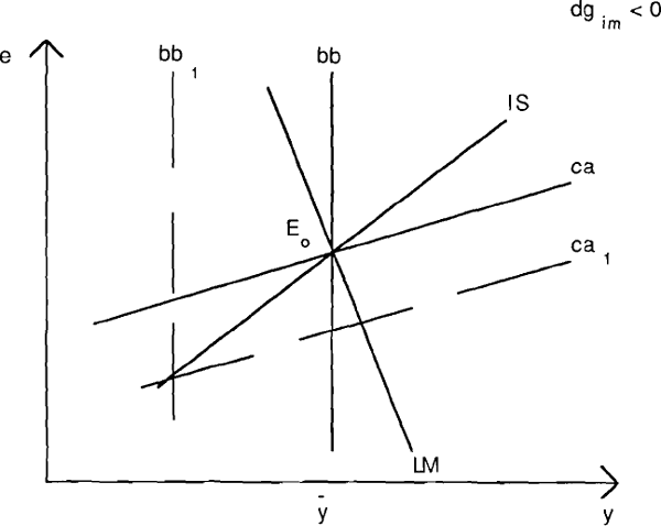
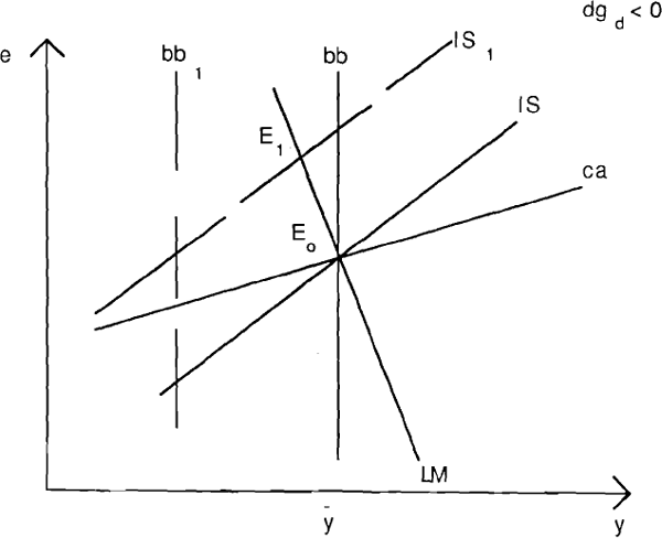
Consider first the effects of a fiscal contraction brought about by cuts in public spending. At an unchanged output level there would be a budget surplus and a current account surplus of the same magnitude as the decrease in spending.[12] But output may respond to the fiscal contraction so the induced tax revenue and current account effects must be taken into account. The composition of government spending is likely to be important here. Figures 3a and 3b illustrate two extreme cases. In the first, all of the government spending cut falls on the imported good. In this case domestic demand is left unchanged and the entire effect of the fiscal policy is felt on the current account which improves one-for-one with the government budget.[13] Figure 3b shows the consequences of the other extreme example in which all of the cut in government spending falls on the domestic good. Now the current account schedule is unchanged whereas the budget balance line shifts to the left as before. Since domestic demand has fallen the IS curve moves to IS1 implying a reduction in output and a currency depreciation. The fall in output leads to an induced loss of tax revenue so the improvement in the government's budget is not as large as before. Similarly, the income reduction limits the room for an expansion in net exports. The final outcome then is an improvement in both of the “twin deficits” but by a smaller amount than in Figure 3a. Whether a one dollar improvement on the fiscal front still brings about an equal current account amelioration can not be ascertained without knowledge of the particular parameters of the model.
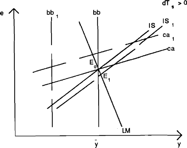
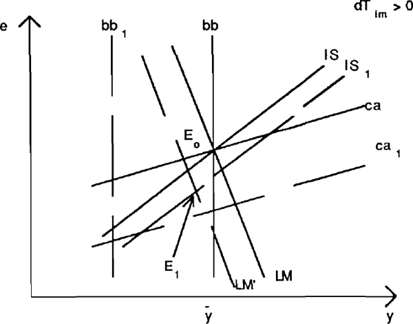
The effects of fiscal consolidation brought about by tax increases are investigated in Figures 4a, 4b, 4c, and 4d. In order to ensure comparability the size of each tax cut is chosen to yield the same improvement in the full employment budget. This means that the bb schedule shifts leftward by the same amount in each one of the figures. Figure 4a illustrates the consequences of an increase in the marginal income tax rate t1. It is clear that the effects are broadly similar to a combination of the two expenditure reductions considered above. Quantitatively, the induced changes in income are going to be smaller than in Figure 3b because a tax increase is less contractionary than an expenditure cut in models of the type considered here.
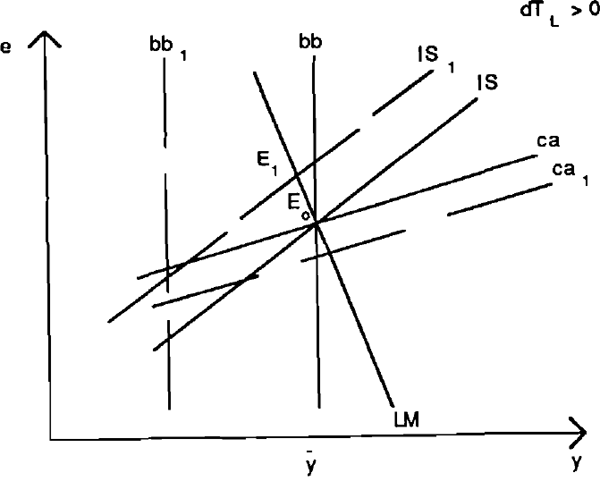
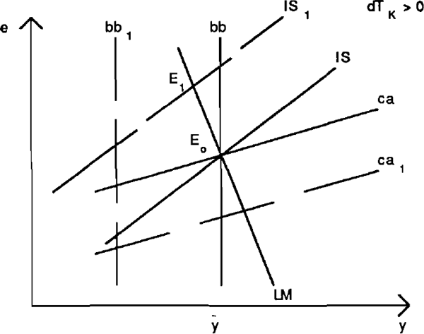
An increase in the corporate income tax rate has two effects. First it reduces disposable income of the owners of capital. This has much the same consequences as the increase in income taxes that we have just examined. In addition, a tax on income from capital is assumed to reduce investment spending for any given level of expected return on capital. This second effect leads to a further reduction in output and a larger currency depreciation than in the previous case. The current account improvement is therefore larger than before whereas the opposite is true for the fiscal balance. This result is perfectly reasonable if one thinks about the current account in terms of the economy's savings-investment balance. For a given improvement in the public sector's fiscal position, a policy that reduces the incentive to invest is going to have a larger influence on the current account than a policy that does not create similar incentives.
Figure 4c illustrates the last argument even more vividly. It shows the consequence of a tax increase that has no direct income effect but that reduces the incentives to save on the part of the private sector. Not surprisingly, this tax increase has an expansionary impact on the economy. The induced increase in tax revenues will add to the direct effects leading to a substantial fiscal improvement. But the reduced incentives to save are actually going to bring about a deterioration of the current account.
The final tax measure we look at is an increase in import taxes. It might be thought that this would have a particularly large impact on the current account since the tax change falls directly on external transactions. But an examination of Figure 4d reveals that this is not the case.[14] The explanation is again to be found most easily by looking at private sector aggregate spending and investment decisions. Increasing an import tax is likely to influence the composition of current spending between domestic and foreign goods but not the aggregate volume. But with total output reacting only by a small amount, the current account will improve only if aggregate spending is reduced. Since this is not the case in this example, external balance will not be sensitive to changes in trade taxes. This conclusion is an example of the general point that expenditure-changing policies have the most direct and quantitatively the strongest influence on the current account whereas expenditure-switching policies are likely to affect the real exchange rate significantly but the current account only indirectly.
Before proceeding to issues that go beyond the formal model presented here it is perhaps useful to summarize the conclusions that have emerged concerning the twin-deficit hypothesis. Most generally stated, we have seen that the particular way in which the budget deficit is reduced is important for the reaction of the current account. Specifically, tax and expenditure changes that influence directly or indirectly the choice between current spending and future spending (i.e. saving) have the largest effects on the current account for a given impact on the public sector's budget. The different implications of a tax increase that discourages investment and one that discourages household saving is the most telling illustration of this basic insight. In the latter case we saw in fact that a budget deficit reduction was associated with a current account deterioration in contradiction to the twin deficit notion. Changes in government expenditures were seen to have effects on the current account and the public sector budget in the expected direction to a large extent independently of the composition of these expenditures. The composition was important for the output and exchange rate effects.
(c) Ricardian Equivalence, Expectations Effects and Other Extensions.
The recognition that the current account balance is closely tied up with savings and investment decisions has led many investigators to argue that theoretical and empirical modeling must pay more attention to the fundamentally intertemporal aspects of these decisions. Doing so raises a number of issues related to how future consequences of current policies affects current behaviour, how policies that are announced but not yet implemented influence the current performance of the economy, and how the accumulation of domestic and foreign debt due to budget and external imbalances affects the economy over time. While a complete discussion of these issues would be far beyond the scope and purpose of this paper, the discussion of the link between fiscal policy and external balance would be seriously incomplete without at least a brief treatment of them.
(i) The Ricardian Equivalence Proposition.[15]
If households are sufficiently forward-looking they might realize that a tax reduction in the current year financed by issue of government debt implies higher taxes in the future when that debt must be serviced and repaid. They might therefore increase their current savings in anticipation of the future taxes. The Ricardian Equivalence Proposition asserts that under certain conditions the entire value of a current tax cut would be saved leading to no increase in consumption and therefore to no increase in economic activity. The current account would also be unaffected since the decrease in public savings would be exactly offset by an increase in private savings. The implication for the twin-deficit hypothesis is that it will matter even more how a budget consolidation is achieved. If it is done by increases in taxes rather than by reduction in expenditures then the benefits for external adjustments are nil.
Of course, the conditions for Ricardian Equivalence to hold completely are rather stringent. For various reasons, households may be less forward-looking than the proposition asserts in which case the savings response to a tax-increase will only be partial. The analysis of the previous section would continue to hold qualitatively although the size of the influences on output, the exchange rate, and the current account would be smaller. In addition, the analysis underlying the Ricardian view relies on taxes being non-distortionary. One of the important conclusions of the foregoing analysis was however, that certain taxes alter incentives to save and invest in which case the Ricardian argument does not apply. The consequences of these kinds of tax changes for the twin-deficit hypothesis therefore remain essentially unchanged.
Although the Ricardian proposition refers to changes in taxes offset by corresponding variations in government debt, it can be shown to have interesting implications for the analysis of changes in government spending as well. As an illustration, consider the case of a reduction in government spending on imports already analysed in Figure 3a. The lower future tax burden implied by the reduced budget deficit is going to induce the private sector to increase its expenditure somewhat. The equilibrium would therefore be located to the south-east of E0 along the LM curve. The outcome in this Ricardian case would be an increase in output, a currency appreciation small current account surplus.[16] While this leaves the qualitative relationship between the current account and the budget deficit unaltered, the one-for-one link between them is broken.
(ii) Direct crowding out or crowding in.
An argument resembling the Ricardian one can be made for government spending as well. If one introduces substitutability and complementarity relationships between government spending on the one hand and private consumption, savings, and investment spending on the other it is easy to generate outcomes that are quite different from those found in the previous section. To give but two examples, consider a transfer of health-care expenditures from the government to the private sector and a reduction in infrastructure investment by the government. In the first case the direct effects on aggregate demand, and hence on overall economic activity and external balance, is likely to be negligible. In the second case on the other hand, the reduction in government investment may lead to an induced fall in private investment resulting in a larger improvement in the economy's external position and a more pronounced slow-down in economic activity than otherwise would have been the case.
(iii) The effects of anticipated future policies.[17]
If financial markets and/or consumers are forward-looking it is important to take into account not only the current stance of economic policies but also the likely future stance. For instance, an announced but not yet implemented cut in government spending is likely to have an immediate expansionary effect for two reasons. Anticipations of future reductions in interest rates (as a result of the future implementation of the expenditure cut) will translate into an immediate reduction in the long-term rate which is likely to boost investment spending. In addition, Ricardian consumers are going to anticipate future tax reductions and therefore increase their current spending. The outcome is likely to be an immediate deterioration of the current account without any direct change in the government's present fiscal position. It is easy to imagine that other examples can be constructed that show important differences between the effects of temporary versus permanent shocks, and between anticipated versus unanticipated shocks.
(iv) Dynamics of debt accumulation.
Accumulation of internal and external debt due to budget- and current account deficits may have effects that are significantly different in the medium to long-term than on impact. The reasons for these differences are not difficult to explain whereas the formal analysis soon becomes cumbersome. Expansion of government debt as a result of budget deficits increases the wealth of the private sector (provided Ricardian Equivalence does not hold completely) and thus aggregate spending. The increasing ratio of government debt to other assets may also require change in interest rates for portfolio-balance reasons. Induced changes in savings and investments may result. Analogous consequences will occur following a build-up of foreign debt. Domestic wealth declines and risk premia may have to be incurred on additional external borrowing. Both factors will influence the medium-term evolution of the economy, notably that of the exchange rate and the current account.
Debt service obligations also give rise to a dynamics of its own. Even if the primary government deficit were to disappear, the outstanding debt would continue to grow at the rate of interest. Similarly, a country's external debt would grow even if its balance of trade were in equilibrium. In order to stabilize the external debt, the trade account would have to be in a surplus equal to the debt service payments. This implies that a short-run currency appreciation brought about by a fiscal expansion may have to give way to a long-run depreciation in order for the necessary trade adjustments to occur. The details of the intervening adjustment path is clearly not easily characterized even in relatively simple analytical models.[18] Numerical simulations may be necessary.[19]
(v) Valuation effects on existing debt.
The formal analysis in parts (ii) and (iii) assumed that the economy initially had no foreign debt and that the government's debt was denominated in domestic currency. While these assumptions greatly simplify the analysis, they are contrary to reality in many cases and they exclude potentially important channels of transmission. Consider the implications of a significant net foreign debt denominated in the foreign currency for the short-run effects of monetary and fiscal policy. We saw above that a monetary expansion will create a trade balance surplus if the elasticities of demand for exports and imports are sufficiently large. As a result of the currency depreciation however, interest payments on the external debt would increase. Potentially, this effect could dominate so that the overall impact on the current account would be negative.[20]
As already noted, similar valuation effects would apply to the government's debt service payments. Any policy or non-policy shock that results in a currency depreciation would increase the fiscal deficit[21] and the debt service component of the current account simultaneously. As a result, a positive correlation between external and internal deficits would automatically be introduced.
(vi) Inflation, the real cost of capital, and the real return to saving.
If nominal interest costs are deductible from profits subject to corporate income taxes then an increase in inflation will reduce the after-tax real cost of capital even if the nominal interest rate fully incorporates the inflation premium.[22] Similarly, the after-tax real return on savings decreases with inflation if nominal interest earnings are subject to income tax. Both of these factors imply a deteriorating savings-investment balance of the private sector as inflation increases. The fiscal balance, on the other hand, may improve especially if bracket creep as a result of progressive income tax schedules increases effective tax rates. The outcome could easily be a current-account deterioration in spite of a reduced public sector deficit.
Footnotes
Taxes on international trade on the other hand, which from the point of view of the elasticities approach would seem to have a strong influence of the current account do not in any very direct way influence the savings-investment balance. [2]
The consequences of a number of important extensions of the basic model are examined in part (c) of this section. [3]
The meaning of the symbols used is given in Table 1. [4]
The most frequent way in which tax policy alters incentives to save is probably through taxes on interest income. This effect could be modeled by making savings (consumption) a positive (negative) function of the after-tax real return on assets held by households. The tax parameter introduced in equation (3) may be interpreted as a proxy for this type of incentive effect. [5]
In a dynamic model this equation would typically be interpreted as a Phillips curve relationship and be written as a differential equation for P. [6]
It is important to note that the LM curve will be steeper (i) the smaller the influence of import prices on the domestic aggregate price level, and (ii) the larger the effect of aggregate demand on the price of domestic goods. [7]
Tariff revenue will increase or decrease with e depending on whether the elasticity of
demand for imports is smaller or larger than unity. The debt service component of
government expenditures varies with the interest rate which in turn varies with e (for a
constant  ). It is assumed that the net effect of these
influences on the budget is small. If some of the government's debt were denominated
in foreign currency a real depreciation would increase real debt service obligations. A
higher level of real income (which increases income tax revenue) would be needed to
balance the budget. In this case the bb line would be positively sloped. Some comments
regarding the implications of valuation effects on existing domestic and foreign debt
will be made in part (c) of this section.
[8]
The term full employment should not be interpreted in the literal sense as an absolute capacity constraint. It should rather be taken to refer to that level of output for which there is neither upward or downward pressure on prices. [9]
The improvement is tempered by the increase in investment spending brought about by the lower interest rate. For the parameters and the time horizon considered here, the interest-rate induced changes in spending will not offset the change in savings. In a situation where the change in output takes some time whereas the change in interest-rate-sensitive spending is immediate, it is possible for the current account to deteriorate in the short-term. [10]
Induced increases in savings as income expands and induced decreases in investment due to a higher real interest rate will not offset this direct effect. [11]
In the original Mundell-Fleming framework this is indeed the final effects of such a policy. [12]
In the figure the equilibrium position of the economy remains at Eo so the level of output and the exchange rate are unchanged. The budget balance and current balance schedules shift to the left and right respectively indicating improvements on both accounts. [13]
Note that both the IS and LM curves shift in this example. The IS curve moves to the right since increased import taxes shift demand onto domestic goods whereas the LM curve shifts to the left because the price level increases due to the higher internal price of imports. The resulting equilibrium may entail an expansion or contraction of output. In either case the currency appreciates and the current account improves only slightly. [14]
Standard references on this topic are Barro(1974) and Carmichael(1982). Mutoh(1985) contains a particularly well-explained open-economy extension. [15]
Note that with Ricardian consumers a debt-financed change in government spending is equivalent to a tax -induced change. The intuition behind the outcome is then clear. The net effect of the reduction in gim is a moderate reduction in total demand (which is what gives rise to the small current account surplus) combined with a switch in demand towards the domestic good (which leads to the currency appreciation). [16]
For an analysis of the evolution of the United States economy in the early eighties emphasizing these effects, see Branson, Fraga, and Johnson(1985). [17]
Note that even the impact effects are likely to be influenced by the properties of the long-run outcome because current expectations may be conditioned by it. [18]
An early theoretical analysis of these issues is contained in Sachs and Wyplosz (1984). Masson and Knight(1986) and Morris(1988). They contain interesting empirical applications as well as simulations relating to the United States, Germany and Japan. McKibbin and Sachs(1988) describe simulation results with a model that takes into account long-run solvency constraints both for governments and for countries as a whole. [19]
In terms of Figure 1, the ca schedule would become steeper than the IS curve in this case. The consequence of this reversal of the relative slopes for the other policy experiments can readily be worked out. [20]
The bb schedule would become positively sloped. [21]
See, for instance, Dews(1988) p. 14. [22]


