RDP 9006: Wage Contracts, Sticky Prices and Exchange Rate Volatility: Evidence from Nine Industrial Countries 2. The Model

(i) The Labour Market

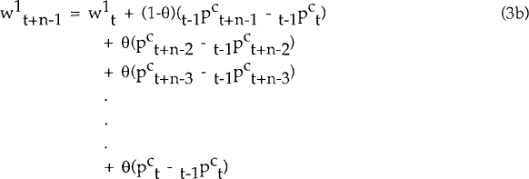
The labour force consists of n cohorts of workers, each of which has a wage contract which lasts for n periods. I assume that all workers in the economy are represented by a single union. Each cohort-specific worker receives the same wage, but differences in wages can arise between workers of different cohorts. Without loss of generality, let the wage contract of the first cohort be in effect from period t through period t+n−1. It is negotiated at the end of period t−1, and so is contingent on information known at that time. The contract is

where π is the “escalator” coefficient and θ is the “catch-up”. w is (the natural logarithm of) the nominal wage, is the nominal wage for period t expected at the end of period t−1 and is the nominal wage that clears the market for workers in cohort 1.

is the log of consumer prices, defined as

where p is the log of domestic producer prices, e is the log of the nominal exchange rate (the domestic price of foreign currency), pf is the log of foreign producer prices and (1 − σ) is the share of imports in consumption.

By assumption, the price level p_t is not known until the end of period t. Employment decisions by firms (which are made at the beginning of each period) are thus made on the basis of the expected real wage for that period – the known nominal wage relative to the expected level of producer prices. The nominal wage for period t, , is set equal to the market-clearing wage for that period. The expected nominal wage for period t+1 is the expected wage for period t, , plus a fraction π of the expected inflation in consumer prices over that period, − . In addition, the contract allows for a fraction θ of the price surprise in the previous period − , to augment wages in t+1. Of course, with rational expectations, this amount has an expected value of zero in t−1, the time of contract negotiation. To keep the model simple I assume that π = 1 − θ, i.e., price changes are assumed to be fully passed onto wages.^[3] However, the extent to which wage inflation reflects anticipated and unanticipated price inflation (the value of θ) is left open to estimation.

Nominal wages for periods t+2…t+n−1 are set in an analogous manner. , for instance, is the wage expected at t−1 for the previous period, , Plus a fraction(1 − θ) of the expected price inflation from t+n−2 to t+n−1, plus a fraction θ of the difference between the price level in t+n−2 and the price level expected at t−1 for t+n−2. In short, the contract sets a sequence of n ex-ante nominal wages , the last n−1 of which are based on expected future inflation. Ex-post nominal wages differ from ex-ante wages because of mistakes in forecasting prices, some fraction of which is passed on to wages. A new contract is signed at the end of period t+n−1, which determines wages in periods t+n through t+2n−l.

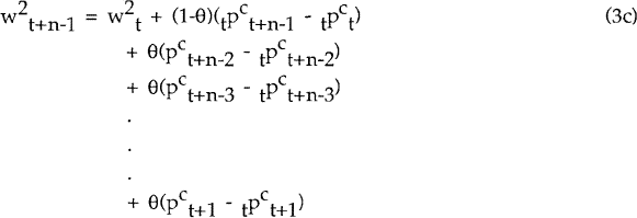
Wages for cohort 2 are set in precisely the same way, except that they are negotiated at the end of period t, and take effect from periods t+1 through t+n. The crucial difference between the wages set for cohorts 1 and 2 (apart from the one period overlap) is the latter are based on information known (and hence expectations formed) at the end of period t. The contracts for cohorts 3…n are set in periods t+l…t+n−2 respectively. They start in periods t+2…t+n−1 and expire in periods t+n+l…t+2n−2.

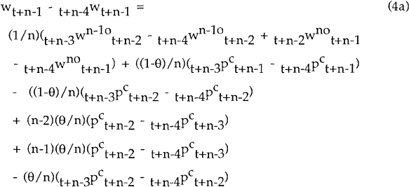
Aggregate wages at time t+n−1 are given by^[4]

where

Taking expectations at t+n−4, and using the law of iterated expectations, we find that

Backdating n−1 periods and re-arranging terms:

Consider the term . This is the change from periods t−3 to t−2 in the market-clearing nominal wage for cohort n−1 expected to prevail in period t−1. This is equal to the change in producer prices expected for that period, plus the expected value of a series of supply and demand shocks which alter the market-clearing real product wage. I assume these shocks to be white noise, and denote the vector of shocks ξ_n−1t. Thus, with E_t−jξ_n−1t = 0, j > 0,

Similarly,

and so

The aggregate wage level at time t is a function of lagged prices, lagged price expectations, expectations of the current wage level and two parameters: the contract length n and the indexation parameter θ. In addition, random shocks η_t, representing wage bargains which occur outside the contracting system, affect the aggregate wage level in every period. These shocks need not be white noise. Indeed we might expect a wage shock in one period to affect wages in subsequent periods; furthermore, the variance of these shocks could well vary from period to period. (These possibilities are taken into account at the estimation stage.) Equation (4e) cannot be estimated in its current form since the expectations variables are unobservable. The conversion of equation (4e) into a form suitable for estimation is discussed in Section 4.

(ii) The Goods Market

I assume that output in each country is produced by a representative firm that competes in the international goods market with other firms/countries. The market structure is monopolistic (so that there is no strategic interaction, as would occur with an oligopoly) with each firm setting the profit maximizing price of its product. However, there exist convex costs to changing prices. Following Giovannini and Rotemberg (1986), the firm's objective function is

where is the price level that clears the goods market at time t+j, δ is a constant discount factor, E_t is the expectations operator, conditional on information at time t and C, (0 < C < 1), represents the cost of changing prices. The first order conditions for this problem can be written as (Giovannini, 1988)

where c = C/[1 + (1 + δ)C], 0 < c < (1/(1+δ)), and _tP_t+1 is the (rational) expectation of p for time t+1, held at time t. Only when c=0 will p_t be equal to its equilibrium (profit-maximizing) price.

Under the assumptions of a Ricardian technology with constant returns and no inputs other than labour, will be a constant mark-up over the nominal wage. This mark-up will be uniform across countries (equation 7a), with the relative price of domestic and foreign goods (the real exchange rate) determined by relative labour costs (equation 7b).

where wf_t is the log of the foreign wage.

Up to a stochastic shock u_t, the equilibrium is characterized by domestic and foreign real product wages being equalized, each measured in its own currency. The competitive equilibrium arises as a special case of this model. If domestic wages are perfectly flexible, then nominal wages at home and abroad will be equalized (in common currency terms) by international competition in the goods market, thus

and so

In addition, if c = 0, then

In the absence of nominal rigidites, PPP will be obtained in the short-run, up to the shock u_t.^[5] If nominal rigidities are present, however, real exchange rates will deviate from their (competitive) equilibrium values.

This is the well-known result established by Dornbusch (1976). If we assume that shocks which cause the exchange rate to deviate from its equilibrium path are unanticipated, then a corollary to that result is that the variance of exchange rate innovations will be larger the more pronounced are the short-run rigidities to nominal wages and prices.

u_t can be thought of as a supply shock, e.g. to productivity, with ε_t a stationary ARMA process. A positive shock to productivity will create a series of current account surpluses. An appreciation of the real exchange rate is then required for intertemporal equilibrium. This occurs via a decrease in p_t and a more than offsetting decrease in e_t

(iii) Foreign Prices

I assume that the log of the exchange rate, e, and the log of the foreign price level, pf, both evolve as random walks:

The foreign wage, wf, is determined as an error-correction mechanism

where τ_t represents disturbances that cause divergences between domestic and foreign wages e.g. country-specific productivity shocks. Complete nominal wage flexibility (w_t = e_t + wf_t) occurs when β = 1. A test of PPP is thus a test of the joint hypothesis that β = 1 and c = 0.^[6]

(iv) Price Dynamics and Persistence

When nominal rigidities are present, the price level p_t is directly affected by four shocks. These are the real shocks u_t, the shocks to foreign prices v_pft, and the shocks to domestic and foreign wages, η_t and τ_t.^[7] I assume that real shocks have a permanent effect on the price level and so u_t is specified to be a non-stationary process. The effect on the inflation rate, however, is temporary. (In the competitive case the price level jumps immediately to its new equilibrium value and the inflation rate changes instantaneously.)

The cost of changing prices imparts serial correlation to the price level; p follows a multivariate autoregressive process when c is not equal to zero. The nominal shocks v_pft, η_t and τ_t have no effect on the steady state price level, but their effects may still be very persistent, depending on the value of c and the process generating _tP_t+1, the expected price level one period hence. Only in the special case of no wage and price rigidities will the wage shocks have no effect on the price level.

Footnotes

This assumption is tested and found to be generally supported by the data; see Section 5 below. [3]

In making this aggregation, I assume that, at any given point in time, all agents in the economy have access to the same information set, and that they use the same expectations-generating mechanism to forecast future prices and wages. I also assume that all n cohorts choose the same θ. This assumption is usually made in the literature on overlapping wage contracts. [4]

I assume that prices and wages are flexible in the long-run and so PPP will eventually be obtained. Thus the transversality condition for the firm's optimization problem is:

View MathML

[5]

Note that equation (8c) does not imply that the domestic wage causes changes in the foreign wage, only that, in equilibrium, domestic and foreign wages will be equalized. Domestic and foreign wages are jointly determined by equations (4e) and (8c). Distortions in either domestic or foreign labour markets will cause β = 1. The terminology “inflexible nominal wages” in this model has the particular meaning “slow convergence of nominal wages between a country and its trading partners”. [6]

The shocks to the nominal exchange rate, v_et, have no direct effect on p_t but they do have an indirect effect via w_t. [7]