RDP 9008: Financial Deregulation and the Monetary Transmission Mechanism 3. Methodology

One way of examining the macroeconomic effects of deregulation is to construct a structural model which reflects the effects of financial liberalisation. However, the precise nature of these structural changes is unclear, and only recently has much thought been devoted to this question; see e.g. Blundell-Wignall et al. (1990). We view this modelling exercise as a topic worthy of future research. In this paper, however, we are content to model the reduced form effects of deregulation. We do this by constructing a four-equation vector autoregression. We estimate this dynamic reduced form and then examine the properties of its moving average representation i.e. the impulse responses and variance decompositions.^[4]

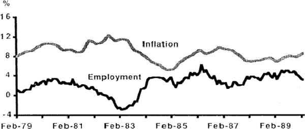
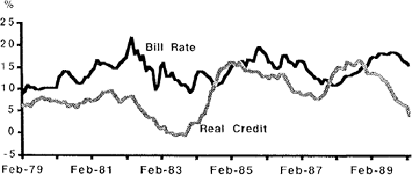
The four endogenous variables that comprise the VAR are the 90-day bank bill rate, the rate of growth of employment, the inflation rate (measured by the growth rate in the Consumer Price Index) and the rate of growth of total real credit in the financial sector. These are graphed in Figures A and B, below.

The 90-day bank bill rate is our proxy for monetary policy. Although monetary policy was implemented essentially through quantity controls pre-deregulation, periods of tightening (easing) were often accompanied by increases (decreases) in interest rates (see Battellino and McMillan, (1989)). In a deregulated environment, changes in cash rates are soon reflected in corresponding changes to the 90-day bank bill rate. Thus we are confident that changes to the bill rate can be interpreted as reflecting changes to the stance of monetary policy both before and after deregulation even though the method of implementing that policy has changed completely. Our measure of credit is the sum of all advances and bank bills. The rate of employment growth is our proxy for real activity.

An important feature of VAR modelling requires discussion. This is that, while a VAR is just a set of reduced form equations, the impulse response functions and variance decompositions are sensitive to the ordering of the variables in the VAR. In effect, a recursive structure is implicitly imposed on the contemporaneous variables in the model, and so the VAR is by no means a mere atheoretical representation of the data. This kind of structure is, of course, very restrictive. There seems to be no completely satisfactory way of resolving this problem but, at the very least, we need to be explicit about the assumptions we are embedding in the model. We place the variables in the following order: the 90-day bank bill rate, the growth of employment, inflation and the growth of real credit. Thus we are assuming that the bill rate is contemporaneously exogenous to the rest of the variables in the model, the bill rate and the growth of employment are together exogenous to the other variables, etc..

Our analysis divides the data into two sub-periods; from 1978:2 to 1984:8 and from 1984:9 to 1990:3. Since deregulation occurred progressively over a number of years, no single date can unambiguously divide the regulated and deregulated periods. Our (admittedly arbitrary) choice is August 1984, the time when all remaining bank deposit controls were removed. This allowed banks to compete for short term funds in the overnight money market for the first time.

Six lags of each variable appear in the VARs, which are estimated consistently and efficiently by ordinary least squares. The parameter estimates, while of no intrinsic interest, are available on request from the authors. The data are monthly and, except for the bill rate, are measured as log differences. Details about data construction and sources can be found in the Appendix.

Footnote

Wold's representation theorem states that a stationary autoregressive process y_t = b(L)y_t + u_t can be written as the vector moving average process y_t = a(L)u_t + E(u_t) where the coefficients of the matrix a(L) are functions of the estimated autoregressive parameters b(L). a(L) at lag 0 is the identity matrix. u_t is the forecast error (innovation) of the autoregression given information at t − 1. In other words, each variable is expressed as the sum of current and past innovations (shocks) of all the variables in the system. The dynamic path of the effects of an innovation to a variable on another variable is the impulse response function. The variance decomposition of the k-step ahead forecast is the proportion of the total forecast variance of one component of y_t+k associated with shocks to the MA representation of another variable. [4]