Relationships Between Major Expenditure Aggregates | RDP 9102: Indicators of Economic Activity: A Review

RDP 9102: Indicators of Economic Activity: A Review 3. Relationships Between Major Expenditure Aggregates

Malcolm Edey and Jill Pleban

March 1991

Download the Paper 384KB

The expenditure aggregates analysed in this section are dwelling investment, business investment (consisting of plant and equipment and construction), consumption, imports and investment in stocks. Graphs 1 to 6 show the growth rates (in year-ended percentage changes) of each component graphed against the growth rate of real GDP.

Graph 1: GDP and Residential Investment

Year-Ended Growth Rates

Graph 2: GDP and Consumption

Year-Ended Growth Rates

Graph 3: GDP and Non-Residential Construction

Year-Ended Growth Rates

Graph 4: GDP and Plant and Equipment Investment

Year-Ended Growth Rates

Graph 5: GDP and Imports

Year-Ended Growth Rates

Graph 6: Change in Stocks and Growth in GDP

Contribution to Year-Ended Growth

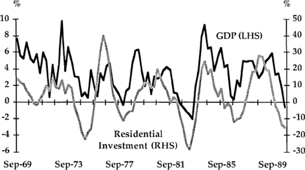
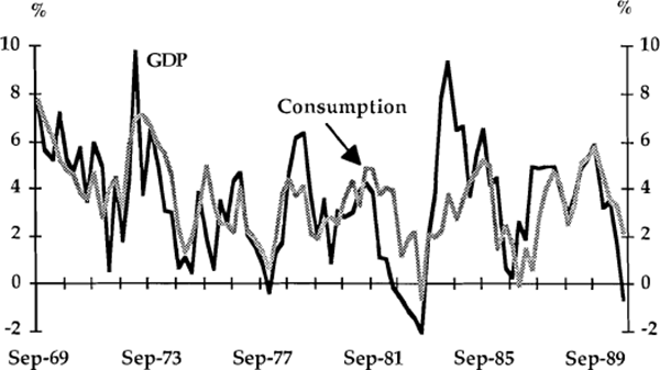
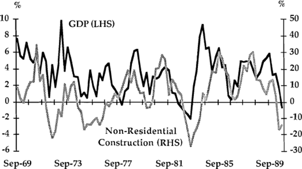
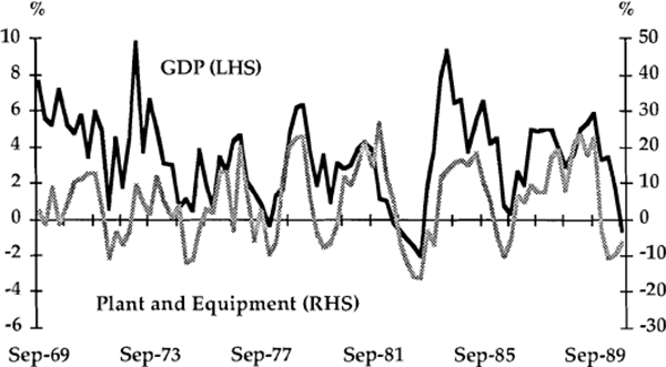
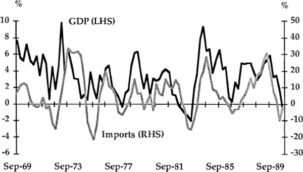
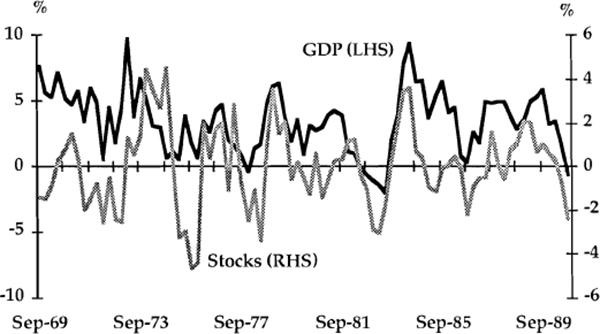
A useful preliminary way of detecting leads or lags between series is to compare the timing of major turning points. In Table 2, twelve turning points in year-ended GDP growth have been identified and where possible, corresponding turning points in the other variables are listed. This preliminary classification, and visual inspection of the graphs, suggest a number of tentative conclusions about timing. First, there is an apparent tendency for dwelling investment to lead the cycle in GDP; turning points in dwelling investment led those in GDP on five occasions, and by up to four quarters. A leading relationship could be rationalised on the basis that housing is probably the sector which reacts most quickly to changes in financial conditions. This would be consistent with the conclusion of Bullock, Morris and Stevens (1989) that interest rates tend to lead the real economy. It might also be argued that housing activity is sensitive to changes in expectations and therefore plays some causal role in generating cycles in activity. Certainly, the amplitude of housing fluctuations is large compared with those of other spending components.

Table 2: Major Expenditure Aggregates:
Comparison of Turning Points
GDP	Res.	BFI	PE	NRC	Con.	Imp.	Stocks
1972(1)	−4	0	0	+1	−1	+2
1973(1)	0	+3	+3	+4	0	+2	+6
1975(1)	−1	−1	−1	−1	−1	+2	+2
1976(4)	−2	0	0		0	−1
1977(4)	0	0	0		0	0	+2
1979(1)	+2	−1	0	−1	−2	−1	+3
1980(1)	0	−1	−1	−1	−2	−2	+1
1981(2)	−3	0	+2	−1	0	0	+2
1983(2)	−1	0	0	0	0	0	−1
1984(2)	0	+4	+4	+5	+5	+1	0
1986(3)	0	−1	−1	+1	+1	0	0
1989(3)	−4	−5	−2	−5	0	−1	−2
Note: The table shows the relative timing of turning points in the year-ended changes in variables shown, relative to that of GDP. A minus indicates a turning point which preceded that of GDP. The abbreviations are residential investment, business fixed investment, plant and equipment, non-residential construction, consumption, imports, and non-farm stocks, respectively.

Consumption (Graph 2) typically follows a much smoother time path than either GDP or any of the other spending aggregates under consideration, presumably reflecting the importance of consumption-smoothing behaviour by households. It also appears that consumption has lagged major changes in income in recent years. A good example of this occurred in the 1982/83 recession when, on a year-ended basis, consumption fell at only one point despite a protracted decline in income. Because consumption represents about two-thirds of total spending, this kind of behaviour has an important stabilising effect, and suggests that consumption spending is unlikely to be an important factor in generating cyclical turning points.

On the basis of the graphs and Table 2, other expenditure components appear to have been either coincident with or lagging real GDP. For example, recent turning points in imports have roughly coincided with those in GDP, following an earlier tendency to lag. Growth in stocks has traditionally been regarded as lagging the cycle, reflecting delayed responses by firms to unanticipated changes in output. One such example occurred with the slowing of growth in 1973/74, which was followed first by a stock build-up and subsequently by a major decline. More recently, however, the contemporaneous correlation between stocks and output appears to have become much closer, perhaps reflecting increased adjustment speeds and improved stock-control methods.

Estimates of the VAR system reported in Tables 3 and 4 unfortunately fail to confirm any robust conclusions about leading and lagging relationships among this group of variables. The tables show estimates when the system contains lags up to two quarters, and four quarters, respectively. Both sets of results imply that there are no significant predictors of GDP growth, including lagged GDP itself. Moreover, there are no variables which lag (or are predicted by) GDP growth, with the surprising exception of residential investment in one of the two cases. There are a small number of significant leading or lagging interrelationships detected among the other variables, but these are generally not robust to changes in the number of lags included in the estimation. For example, housing and business investment are significantly related in both models, but in opposite directions. It seems likely that these negative results are due at least partly to a lack of power in the tests, rather than to a genuine absence of underlying relationships; estimates of more restricted systems described below do suggest that some leading and lagging relationships involving GDP growth can be identified.

Table 3: VAR System with Two Lags
	Res.	NRC	PE	Con.	Imp.	Stocks	GDP
Res.	14.9^*	1.0	2.1	0.1	1.8	0.9	0.2
NRC	1.0	1.7	2.7	2.2	0.7	1.0	1.3
PE	4.0^*	1.3	3.9^*	0.2	2.0	2.9	0.1
Con.	1.1	0.2	0.4	1.5	1.1	0.1	2.1
Imp.	4.2^*	1.2	1.9	2.5	0.0	0.5	0.5
Stocks	2.3	0.0	0.1	1.9	2.2	4.6^*	0.1
GDP	2.3	0.3	0.2	1.0	1.7	1.3	2.5

Table 4: VAR System with Four Lags
	Res.	NRC	PE	Con.	Imp.	Stocks	GDP
Res.	5.8^*	1.5	2.9^*	0.7	1.1	1.1	4.3^*
NRC	0.9	1.4	2.2	0.7	0.7	0.7	0.6
PE	2.0	1.5	2.3	0.7	0.7	0.8	0.5
Con.	1.3	0.1	0.8	1.2	2.0	0.6	1.0
Imp.	1.9	1.9	2.0	1.2	0.1	1.1	0.9
Stocks	0.5	1.0	0.9	1.6	1.5	6.3^*	1.0
GDP	1.2	0.2	0.6	1.2	0.4	0.5	1.4
Note: The tables show F-statistics for the null hypothesis that lag coefficients of the right-hand variables are jointly zero. The estimation period is 1969(3) to 1989(2). Asterisks denote significance at the 5 per cent level. All variables are measured in quarterly log-differences.

Tables 5 and 6 present results based on bivariate VARs and simple correlation coefficients. It should be stressed that there is no claim that these represent causal systems, since the implied systems are clearly incomplete; they are simply presented as an alternative way of describing the data, showing whether or not each particular variable contains information about GDP, given that other information is ignored. Once again, conclusions depend on the number of lag lengths considered. When the systems are estimated with only two lags, one obtains the results that housing leads GDP, while consumption and business investment (mainly the construction component) lag. This is true of both the VAR and correlation estimates. However, the results are very much weakened when the number of lags is extended to three or four; in most cases the apparent “causation” either disappears or becomes bi-directional.

Table 5: Bivariate VARs
	2 lag model		3 lag model		4 lag model
	GDP	Res.	GDP	Res.	GDP	Res.
GDP	3.3^*	3.2^*	2.2	1.9	2.5^*	2.3
Residential	0.2	13.3^*	2.4	8.7^*	2.2	11.5^*
	GDP	NRC	GDP	NRC	GDP	NRC
GDP	1.8	1.1	1.7	1.5	1.9	1.3
NRC	2.9	2.0	1.8	1.1	1.6	0.6
	GDP	PE	GDP	PE	GDP	PE
GDP	2.6	0.9	1.9	0.6	1.9	1.4
PE	1.1	1.6	0.7	1.3	0.7	1.5
	GDP	Con.	GDP	Con.	GDP	Con.
GDP	2.2	1.5	1.5	1.7	1.9	1.6
Consumption	4.3^*	2.2	2.9^*	1.9	2.0	1.5
	GDP	Imp.	GDP	Imp.	GDP	Imp.
GDP	2.3	1.9	1.9	1.4	1.9	1.0
Imports	1.3	1.6	1.3	1.1	0.7	1.5
	GDP	Stocks	GDP	Stocks	GDP	Stocks
GDP	1.9	1.8	1.5	1.6	1.3	0.8
Stocks	0.4	20.5^*	3.9^*	13.1^*	2.0	9.8^*
Note: Data periods and notation are the same as in Tables 3 and 4.

Table 6: Correlations with GDP
	Lag in quarters
	−4	−3	−2	−1	0	1	2	3	4
Residential	−0.13	0.02	0.19^*	0.14	0.33^*	0.13	0.05	0.26^*	−0.13
BFI	−0.27^*	0.02	−0.05	0.13	0.31^*	0.20^*	−0.05	0.11	0.06
NRC	−0.15	0.08	−0.08	0.15	0.05	0.27^*	0.07	0.05	0.11
PE	−0.25^*	0.06	−0.02	0.07	0.35^*	0.11	−0.09	0.12	0.00
Con.	−0.13	0.10	−0.16	0.09	0.22^*	0.26^*	−0.05	−0.03	0.05
Imports	−0.13	−0.05	−0.12	0.11	0.20^*	0.17	0.15	0.12	−0.06
Note: The table shows simple correlation coefficients of each variable against lags of GDP. Thus, for example, a significant negative lag indicates that the variable is correlated with future GDP. Asterisks denote significance at the 5 per cent level.

Drawing together the above results and discussion, it is clear that only the most restricted of the statistical methods support the conclusions taken from visual inspection of the data; these were that housing tends to lead the cycle while consumption, construction, and perhaps imports, lag. The negative results obtained from the larger unrestricted VARs suggest a degree of caution in accepting these visual impressions because the leading and lagging relationships may not be particularly strong or reliable. They also suggest that those relationships are “partial” in nature; for example, housing investment does contain useful information about future GDP, but it is only statistically significant when all other current information variables are ignored. A final conclusion to be drawn is that one should be wary of putting strong interpretations on the results from any individual statistical procedure. Results from the large VAR systems in particular seem highly sensitive to changes in design.