RDP 9306: Inventories and the Business Cycle 2. A Model of Inventory Investment

In this section we present a simple model of inventory investment. The model allows an exploration of the factors that determine the relationship between inventories, productivity, output and sales. It is similar in spirit to the model presented in Blanchard and Fischer (1989).

The focus of the model is on a single firm's cost-minimisation problem. It is assumed that the future demand for the firm's product is uncertain, the firm is risk-neutral and that production decisions must be made before demand is known. The firm holds inventories to meet unexpectedly high demand and to smooth production. The problem for the firm is to minimise the present discounted value of its costs given expected demand. The firm's expected costs have two components. The first is standard production costs. The second component is the cost of having inventories depart from a target level. Holding too many inventories leads to undesirably high storage costs while holding too few inventories creates an unacceptably high probability of being unable to meet demand.

Given this structure, the firm's problem can be written as follows:

where:

Y_t denotes production in period t, S_t denotes sales in period t and I_t denotes inventories in period t. Desired inventories in period t are given by , θ is the discount rate, u_t a productivity parameter and Ω_t denotes the information set. The larger is u_t, the higher is productivity and the lower is marginal cost.

The first term in (1) represents the convexity of the cost function. The larger is γ the faster marginal cost increases with increases in production.^[4] If γ is zero, marginal cost is constant. The second term captures the costs associated with inventories being away from their target level. These costs include holding costs and costs associated with being unable to meet unexpectedly high demand. The larger is β the greater are these costs. The target level of inventories is equal to a linear function of expected sales. This is given in equation (2) where δ is the target ratio of inventories to sales. Equation (3) is the inventory accumulation identity and equation (4) defines the information set. Note that when deciding the level of current production the firm knows its current level of productivity but it does not know the current level of sales.

Taking expectations of equation (3) and re-arranging we can define actual production in period t by:

Further, it can be shown that the expected stocks at the end of period t are defined by:

Here, 0 ≤ λ ≤1 and is a function of γ, β and θ. If γ = 0 (that is, marginal cost is constant and production smoothing is not important) then λ = 0, while if β = 0, λ = 1.

2.1. Productivity Shocks

We are now able to explore the impact of shocks to productivity on inventories and output. First, suppose that the firm observes a favourable shock (ε_t) to productivity and that productivity follows the following process:

where ρ ≤ 1. If ρ < 1, then shocks to productivity are only temporary while if ρ = 1 shocks to productivity represent permanent changes. For ease of exposition, initially assume that the increase in productivity does not affect expected sales. In this case, production and inventories will be expected to increase by:

A productivity shock will lead to a positive correlation between changes in production and inventories. The intuition is straightforward. With productivity temporarily high, the firm wishes to increase production while costs are temporarily, relatively low. It will store this extra production as inventories and sell it when productivity and production are below normal levels.

The extent to which inventories increase in response to a productivity shock depends upon the need to smooth production, the discount rate and the persistence of the shock. To remove complications caused by the discount rate assume that θ = 0. In this case, the greater is the cost of holding excess inventories, the smaller will be the increase in inventories following the productivity shock. Similarly, the greater is the convexity of the cost function, the smaller will be the increase in output and inventories. Finally, the size of the inventory response is decreasing in the persistence of the shock. In the limit if ρ = 1, (that is, the improvement to productivity is permanent) there will be no increase in inventories as the lowering of costs is expected to be permanent. There is no advantage in producing more today as production costs are expected to be permanently lower.

The above discussion assumes that sales are unaffected by the productivity shock. However, higher productivity will increase income in the economy and this should lead to an increase in sales. Thus, a more general model in which sales are a function of permanent income would predict that innovations in inventories, driven by productivity shocks, should be positively correlated with both innovations in output and sales.

2.2. Demand Shocks

We now consider the effect of shocks to demand. To do this assume that sales are generated by the following process:

where ϕ ≤ 1. Given the assumption that production must be determined before sales are known, any unexpected change in demand is, in the first instance, reflected in inventories. Thus, in the case of shocks to demand there will be a negative correlation between innovations in demand and innovations in inventory investment. Inventories are essentially used as a buffer stock.

Setting the productivity parameter to zero, the relationship between the following period's output and the current shock to sales is given by:

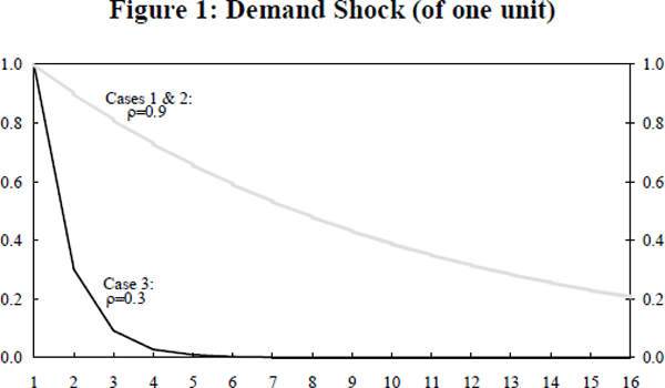
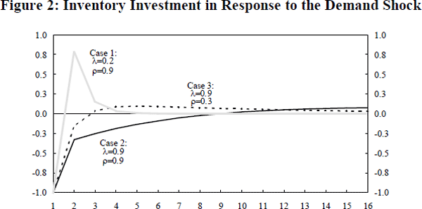
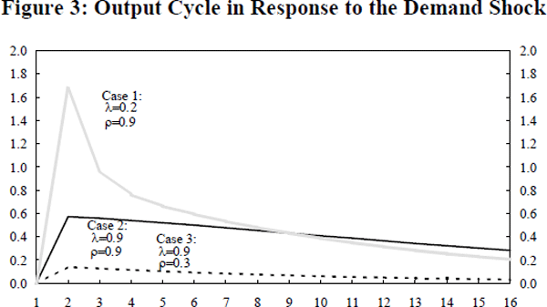
By iterating forward, it is possible to calculate the path that inventories and output take through time in response to the shock. From the path of inventories, the level of inventory investment can be calculated. This path depends on the parameters of the model. In Figures 1 to 3 we present the demand cycle, the inventory cycle and the output cycle, respectively, for three sets of parameter values. In each case the discount rate is set to zero, ξ=1 and the initial demand shock is one unit. In the first two examples the demand shock is quite persistent (ρ = 0.9) while in the third example it shows little persistence (ρ = 0.3). The three paths for inventory investment are distinctly different. In case 1 inventory investment amplifies the cycle in output while in cases 2 and 3 it tends to dampen the output cycle.

First consider case 1 in which shocks are relatively persistent and the need for production smoothing is relatively small (ρ = 0.9 and λ=0.2). In this case, faced with an unexpectedly high demand in period one and unexpectedly low inventories, the firm wishes to re-establish its desired level of inventories in the following period. With little convexity in the cost function, the extra production needed to satisfy higher demand and to rebuild inventories increases marginal cost by a relatively small amount. Thus, the firm is willing to substantially increase output to rebuild stocks. The inventory cycle thus amplifies the output cycle. This can be seen in Figure 3.

Now consider an increase in the convexity of the cost function so that production smoothing is very important (Case 2: ρ=0.9 and λ=0.9). In this case, inventory disinvestment not only occurs in the period in which demand is unexpectedly high, but it continues for a number of periods. The cost function is so convex that some of the higher demand is met for the following nine periods out of inventories.

This reflects the fact that even though demand is high, the firm is only willing to increase production by a very small amount because marginal cost increases very quickly. It is only after 10 periods when demand is two-thirds of the way back to its original level, that inventory investment again becomes positive and stocks begin to increase. In this particular case, the inventory cycle tends to dampen the output cycle. This can be seen in Figure 3.

The third case presented is where there is little persistence in shocks to demand and where production smoothing is quite important (ρ = 0.3 and λ=0.9). In this case, there is only a small cycle in output. Some relatively small inventory disinvestment takes place after the initial shock, followed by a period of sustained but gradual accumulation of inventories. Here the production smoothing is important in stopping the firm from instantly rebuilding its inventories following the initial increase in demand.

There are two important points to be gained from the above examples. First, if the business cycle is driven by demand shocks and inventories act as a buffer-stock, there should be a negative contemporaneous correlation between innovations in inventory investment and innovations in demand. Second, the extent to which the inventory cycle will be important in driving the business cycle depends upon the persistence of shocks to demand, on the extent to which firms wish to smooth production and on the costs of holding inventories. If marginal costs are constant and production smoothing is unimportant, the inventory cycle will amplify the business cycle. If, in contrast, marginal costs increase quickly with production, the inventory cycle is likely to reduce the amplitude of the business cycle.

Finally, we consider the impact of improvements in inventory management techniques on the inventory and output cycles. The implementation of improved techniques might be expected to reduce the target ratio of inventories to expected sales (that is, to reduce δ and thus increase ξ). From equation (10) it can be seen that an increase in ξ reduces the output response for any given shock to demand. The intuition is simple. Given an increase in demand, the amount by which desired inventories increase, depends on the target stocks to sales ratio. The higher the ratio, the greater will be the desired increase in inventories, and thus the greater the desired increase in output. This suggests that any improvement in inventory management techniques that reduces the target stocks to sales ratio should see unexpected changes in demand produce smaller inventory and output cycles.

2.3. Expected Changes in Demand

Above we considered unexpected shocks to sales. Now we consider the case in which the firm actually expects an increase in sales. Again, suppose that sales follow the process given in equation (9) but that the firm expects that in the next period η_t will equal one, rather than zero. In this case if the discount rate is zero, the firm will initially change production by the following amount:

This expression can be greater than, or less than one (the size of the expected demand shock). Thus, expected inventories and expected demand may be either positively or negatively correlated. If production smoothing is relatively important (ξ>ρ), then the firm will be willing to meet some of the extra demand out of inventories. As a result, output will rise by less than the increase in demand and inventories will fall. However, the greater is the persistence of the expected demand shock (the higher is ρ) the lower is the likelihood that the expected increase in demand will be associated with a fall in inventories.

The intuition for this result is as follows. As expected sales increase, the desired level of stocks also increases. Now suppose that the shock to demand is expected to last only one period and that marginal cost increases rapidly with output. In this case, the achievement of a higher stock level to reduce the probability of running out of stock would lead to a substantial increase in production costs. The firm is unlikely to be willing to incur these costs. Instead, it tolerates some run down in inventories and an increase in the probability of running out of stock. In contrast, if marginal costs increase by only a small amount when output increases, the saving in production costs from tolerating an increase in the probability of running out of stocks is small. Consequently, the firm will be more willing to increase output. In addition, the more permanent is the increase in sales the greater is the increase in the probability that stocks will be depleted if output is not expanded.

As was the case for unexpected changes to demand, the output response to an expected change in demand is decreasing in the target ratio of stocks to sales (this can be seen by recalling that ξ is a decreasing function of the stocks to sales ratio (δ)). If the stocks to sales ratio falls, the desired inventory response following an increase in expected demand is smaller, and as a result, the output cycle is less pronounced.

Footnote

As in Blanchard and Fischer (1989) we ignore linear terms as they simply affect the constant term in the solution. [4]