RDP 9410: An Empirical Examination of the Fisher Effect in Australia 4. Interpreting Inflation Forecasting Equations

The conclusion from the preceding empirical analysis is that it is reasonable to assume that there is a long-run Fisher effect in Australia but not a short-run Fisher effect. This characterisation of the inflation and interest rate data along with the assumption of rational expectations can be used to provide a straightforward interpretation of when we will be likely to see estimated β coefficients substantially above zero in the inflation forecasting equation (1). As in Mishkin (1990), we can derive an expression for the coefficient β in the inflation forecasting equation (1) by writing down the standard formula for the projection coefficient β, while recognising that the covariance of the inflation forecast error with the real interest rate, rr_t, equals zero given rational expectations. The resulting formula for the predicted value of β is:

where,

= σ[E_t(π_t)]/σ[rr_t] = the ratio of the unconditional standard deviation of the expected inflation rate to the unconditional standard deviation of the real interest rate.

ρ = the unconditional correlation coefficient between the expected inflation rate, E_t(π_t), and the one-period real interest rate, rr_t.

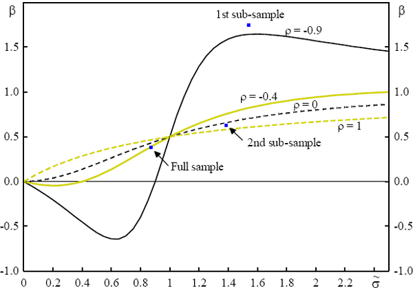
The equation above indicates that β is determined by how variable the level of expected inflation is relative to the variability of the real interest rate (represented by , the ratio of the standard deviations of E_t (π_t) and rr_t), as well as by the correlation of the expected inflation rate with the real interest rate (ρ). Figure 2 shows how β varies with and ρ.

As we can see in Figure 2, when the variability of the level of inflation is greater than the variability of the real interest rate, so that is above 1.0, the β coefficient will always exceed 0.5 and will increase as increases. If inflation has a unit root and thus does not have a stationary stochastic process, as is consistent with the empirical evidence in this paper, then its second moment is not well defined and the standard deviation of the inflation level will grow with the sample size. On the other hand, the existence of a long-run Fisher effect implies that even if inflation and interest rates have unit roots, the real interest rate has a stationary stochastic process and will have a well defined standard deviation that does not grow with the sample size. Hence when we are in a fairly long sample period in which inflation and interest rates have unit roots, the existence of a long-run Fisher effect means that will be likely to exceed one and produce a value of β substantially above zero.

The above interpretation helps explain why we see the strong correlation between interest rates and future inflation that we found for both pre and post 1979 sample periods in Table 1. To see this more clearly, we can calculate estimated values of and ρ. We do this by using the procedure outlined in Mishkin (1981), where estimates of the real rate, rr_t, are obtained from fitted values of regressions of the ex-post real rate on past inflation changes and past interest rates.^[12] Then the estimated expected inflation is calculated from the following definitional relationship,

Finally estimates of σ[E_t(π_t)], σ[rr_t], and ρ are calculated from the estimated E_t(π_t) and rr_t.

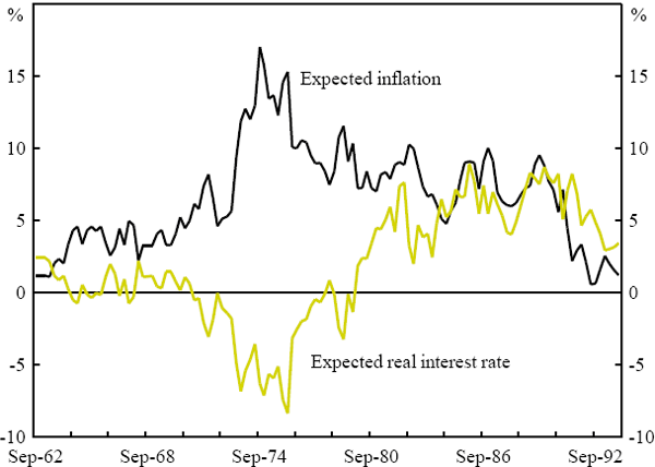
Figure 3 shows the resulting estimates of expected inflation and real interest rates, E_t(π_t) and rr_t respectively, while the estimates for each of the sample periods are shown in Figure 2. As we can see from Figure 3, the variability of expected inflation is greater than that of the real interest rate in the pre 1979 period, resulting in a pre 1979 of 1.5. Also as is visible in Figure 3, expected inflation and the real rate are highly negatively correlated with a correlation coefficient of −0.9. As Figure 2 indicates, the predicted β using these values of and ρ for the pre 1979 sample period is substantially greater than one, which is what we found in Table 4.^[13] For the post 1979 sample, expected inflation continues to be more variable than the real rate leading to an estimate of of 1.4, while there is little correlation of expected inflation and real rates, ??= 0.2. The slightly lower and more positive ρ leads to a predicted ? which is lower in the post 1979 sample than in the pre 1979 sample, although it is still greater than 0.5 because is greater than one. Our analysis thus explains why the estimated β coefficient in Table 1 falls in going from the pre 1979 to the post 1979 period.

Figure 3 also shows that estimated real interest rate had a dramatic upward shift after 1979, a result which has also been found in other OECD countries.^[14] This shift in the real interest rate causes the standard deviation of the real rate to be higher for the full sample period than it is for either of the sub-periods, thus leading to a for the whole sample of 0.9. The less than one means that β should drop below 0.5 and this is again what is found in Table 1. We see that the pattern of estimated β found in Table 1 is exactly what our model predicts.

Footnotes

The estimates described in the text were generated from OLS regressions in which the ex-post real rate, eprr_t, was regressed on i_t, and on π_t−1 and π_t−2. The estimated values of and ρ are robust to different specifications of the regression equations. [12]

This is consistent with the results of Carmichael and Stebbing (1983). [13]

See Cumby and Mishkin (1986). [14]