RDP 9503: Monetary Policy Goals for Inflation in Australia A Framework
March 1995
- Download the Paper 86KB
In this section, we develop a simple macro model of the Australian economy in order to examine the trade-off one might expect between output and inflation variability, given the sort of shocks which hit the Australian economy. Consequently we can assess the likely variability in output and interest rates concomitant with maintaining medium-term inflation at a nominated level.
The model of the economy consists of simple equations for output and inflation, and a reaction function for short-term interest rates (the instrument of monetary policy), which is derived from an objective function for monetary policy. This model is simulated, subject to sets of shocks of zero mean but of the same variance as those in the model's estimation period (1980–1994). Each simulation generates a path for inflation and output, and from the collection of these results the inflation/output variability trade-off is derived.
4.1 The Model
The model consists of the following objective function and two reduced-form equations for output and inflation.
The objectives for monetary policy are to keep (quarterly) inflation (?t) close to
the target level for inflation  , and output (yt)
close to its trend or potential level
  . The parameter ? reflects the
relative weight placed on the two objectives. When ??= 0, monetary policy focuses entirely on
maintaining inflation close to its target level, whilst when ??= 1, monetary policy focuses
completely on maintaining an output gap as small as possible. A target level for quarterly
inflation of 0.5 per cent was chosen, consistent with an annual target rate of inflation of
around 2 per cent.[8]
The central bank minimises this objective function by choosing a path of real short-term
interest rates  .
The first order conditions (derived by minimising the objective function with respect to each
interest rate) define a monetary policy reaction function, in which the interest rate depends on
the expected future paths of inflation and output.
The final term in the objective function ensures that the path of interest rates is not too unstable. A value for ?, the weight on interest-rate smoothness, of 0.01 was chosen which gives a standard deviation of real interest rates in keeping with historical values for the Australian economy.
4.2 The Equations
The output equation is based on the work by Gruen and Shuetrim (1994). Output growth depends on monetary policy, the weather and foreign output. The equation was estimated using quarterly data from March 1980 to September 1994.
The dependent variable is quarterly GDP growth. Monetary policy (measured by the real cash rate, R) affects output with a lag of two to five quarters. This is consistent with prior evidence of the time lags in the effect of monetary policy on output. The Southern Oscillation Index (SOI) captures the effects of weather.[9] When this variable is positive, rainfall is higher, which has a stimulatory effect on growth in the rural sector and from there on the general economy. The final three variables capture the influence of foreign output. The first of these three variables (together with the lagged level of Australian GDP) generates the co-integrating relationship between Australian and foreign (OECD) output (YF) identified by Gruen and Shuetrim (1994).[10] The final variable measures the short-run effect of variations in foreign output on Australia's GDP growth.
 = 0.45 = 0.45
|
S.E. of estimate = 0.720. |
t-statistics are in parentheses. The coefficient on R is the mean coefficient on lags 2 to 5 of the real cash rate. The number in square brackets is the p-value on the F-test of joint significance. et is a white noise error term. |
|
The inflation equation is estimated by regressing the quarterly rate of inflation on its own lags, the growth rate of (tariff-adjusted) import prices, and the output gap. The output gap is the difference between the level of GDP and trend GDP derived from the above output equation, when all explanatory variables are set at their long run averages. In this model, trend output grows at 0.87 per cent per quarter, or around 3.5 per cent on an annual rate, which was about the average rate of growth of the Australian economy in the 1980s.
Lags of inflation are included to capture the effect of inflation expectations. The sum of the coefficients on the lags of inflation and import prices are not significantly different from 1. Accordingly, the equation is estimated with this restriction over the period March 1980 to September 1994. The estimated lag structure suggests that inflation expectations are highly responsive to actual inflation. The sacrifice ratio in this equation is 3.7, a little higher than the range of results for Australia presented in Stevens (1992), but not especially high by international standards.
 = 0.81 = 0.81
|
S.E. of estimate = 0.320. |
There are three exogenous variables in this system: the weather (SOI), foreign output, and import prices. To simulate the economy, it is necessary to have data generating processes for these exogenous variables. The weather was estimated as an AR(3) process. Foreign output was assumed to be a trend-stationary process, with a trend growth rate of just under 1 per cent per quarter. Import prices are assumed to rise with domestic inflation, but can be pushed off this trend by the stance of monetary policy or import price shocks. This exchange rate channel of monetary policy (not shown here) is calibrated so that the impact on inflation is slightly less than the impact of policy via the output channel over a period of two years, which is consistent with other work on the monetary policy transmission process in Australia. This offsets, to some extent, the fact that the coefficient on import prices looks quite low relative to other empirical findings for Australia. This channel takes effect with a lag of one quarter and has a stronger up-front effect on inflation than the output channel.
There are five shocks which can hit the economy each period: a shock to import prices, a shock to foreign output, a shock to the weather, and shocks to output and inflation not covered by the first three channels. All the shocks are uncorrelated contemporaneously and across time. We interpret the price equation shock and the import price shock as “supply” shocks, and the others as “demand” shocks. There are no shocks to potential output, which in this model is a deterministic process.
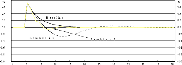
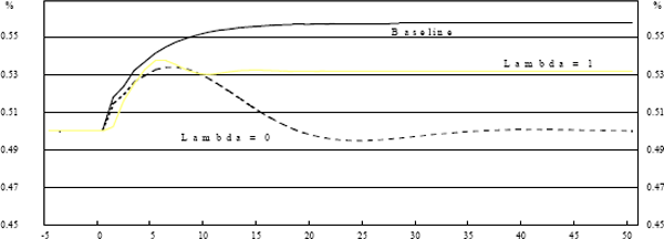
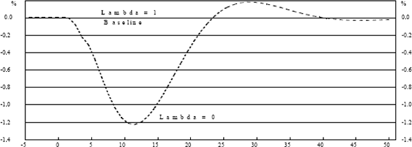
To illustrate the model's properties, we show the responses to a single, one-standard deviation shock to output (demand) and price (supply) in Graphs 2–5.


Lines for λ = 0 and λ = 1 are shown, together with a “baseline” case where there is no policy response to the shock at all.
A positive output shock opens an output gap. Since the shock lasts only one period, the gap will subsequently close as the long-run properties of the model assert themselves. A policy response seeking to minimise output variance will close the gap faster. Either of these alternatives leave inflation permanently higher. The policy response which seeks to minimise inflation variance creates a negative output gap, so that the cumulative sum of the gaps is zero, thus bringing inflation back to its original level.
In the case of a price shock, there is no mechanism to bring inflation back in the absence of policy response. Totally output-focused policy does not respond because there is no output gap. Totally price-focused policy pushes output temporarily below potential to return inflation to target.
4.3 Simulating the Economy
The economy is initially in a steady state, where the real cash (overnight) rate is at its model-determined equilibrium level of 4.6 per cent, inflation is at its target rate of 0.5 per cent per quarter, and output is growing at trend. The economy is then subjected to a set of shocks in each period, with mean zero and standard deviation equal to the relevant estimated standard error in history. For example, the output equation is subject to shocks drawn from a normal distribution with a mean of zero and a standard deviation of 0.72. There are no shocks to import prices, which abstracts from one important potential supply shock, but there are still shocks to inflation (other supply shocks which would be hard to identify in practice), output, foreign output and the weather.
The policy-maker is assumed to know perfectly the structure of the economy described in the equations above, but only learns about the shocks in the period that they occur.[11] In each period, the policy-maker chooses the optimal present level and future path for interest rates to minimise the objective function. The model is run over a 25-year period.
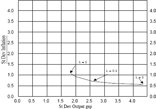
To generate the trade-off curve, the value of the trade-off parameter???is varied from 0 (where there is no weight on output) to 1 (where there is no weight on inflation). For each value of ?, the deviations of inflation from its target value and output from its trend are calculated. This exercise is repeated for 50 sets of shocks, and the mean values of the 50 realisations of the standard deviations for inflation and the output gap are calculated.
Graph 6 shows such a trade-off curve. The empirical magnitudes in this trade-off are not dissimilar to those in some studies for the US – for example Lebow et al. (1992). The graph shows, as expected, that as the weight is increased on the output objective, the variability of the output gap is decreased but the variability of inflation is increased. The trade-offs become increasingly flat: continued reductions in price variability appear to come at increasing cost to output variability and vice versa. When complete weight is placed on prices in the objective function, the standard deviation of the inflation rate is still 0.64 per cent per quarter. This is about double the standard error of the estimate in the inflation equation, and reflects the shocks to other variables (as well as the lag in adjusting policy, and in policy having its effect). This illustrates the point made in Part 3 of the paper about forecast errors.

| ? | Output gap | Inflation* | Interest Rates |
|---|---|---|---|
| 0 | 4.03 (0.80) |
0.64 (0.11) |
5.79 (1.33) |
| 0.025 | 3.02 (0.49) |
0.69 (0.13) |
4.10 (0.92) |
| 0.05 | 2.67 (0.42) |
0.73 (0.15) |
3.64 (0.81) |
| 0.1 | 2.32 (0.35) |
0.79 (0.18) |
3.31 (0.69) |
| 0.2 | 2.01 (0.29) |
0.87 (0.23) |
3.18 (0.57) |
| 0.4 | 1.75 (0.23) |
0.98 (0.31) |
3.31 (0.48) |
| 0.8 | 1.58 (0.19) |
1.15 (0.44) |
3.69 (0.45) |
| 1 | 1.55 (0.19) |
1.21 (0.50) |
3.87 (0.45) |
Standard errors of estimates in brackets. |
|||
Interest rate variance increases for extreme values for λ: very ambitious goals for minimum price or output variability increase the activism of policy, which in this model works to the detriment of the performance of the other variable. This high interest rate variability is most pronounced in the case of λ = 0 (maximum weight on inflation), which one would expect: given the very responsive nature of inflation expectations, a shock to inflation must be countered quite quickly, otherwise it translates quickly into inflation being permanently away from target.
There are, of course, a large number of caveats to this exercise. The model is simple, and numerous complexities of the real world are not captured. This is particularly so with regard to its treatment of the exchange rate. While there is an exchange rate channel of monetary policy, we have not captured the volatile nature of the exchange rate, and its response to shocks to the terms of trade, as well as we would like.
The results are also particularly vulnerable, inevitably, to the Lucas critique: if over time, the regime of inflation targets becomes more credible, one would expect the parameters of the two equations to change. This may be particularly relevant to price expectations. In the extreme, if the inflation target was perfectly credible, shocks to inflation would require a minimal response from monetary policy as inflation expectations would be unchanged. An upward (or downward) movement in inflation would be perceived to be a result of (temporary) inflation shocks rather than a change in the tolerance of the central bank for higher or lower inflation. Inflation would be stationary around the level of the inflation target, in contrast to the current aggregate supply equation, where tight monetary policy (which causes output to fall below trend) is necessary to bring inflation back to its target level after a positive shock. This implies that the sacrifice ratio would decline, with a smaller rise in interest rates (and hence a smaller decline in output) required to reduce inflation.[12] In summary, the trade-off curve above would move in towards the origin.
The speed with which credibility is established may also be dependent on the initial choice on the curve, so that the long-run position of the trade-off curve may be path-dependent. A point chosen which entails lower inflation variability at the cost of higher output variability in the short term might be beneficial in establishing credibility, which would permit lower variability for both inflation and output in the longer term. On the other hand, too ambitious an initial objective for inflation variance might not be credible if there is a risk of general support for the regime being eroded by high output volatility.
Conceding all these points, only very tentative conclusions can be drawn from these preliminary results. We offer two observations.
The first is perhaps stating the obvious, but bears repeating anyway. It is that on the basis of our present state of empirical knowledge of the economy's structure and of the shocks to which it has been subject in the past, it is possible to conceive of a forward-looking monetary policy regime which both ties down the long-run average inflation rate effectively, and allows some response to output considerations in their own right (ie a point in the middle of the curve in Graph 6). (It is worth stressing that the output fluctuations here are around a given potential path; it is assumed that policy-makers have an accurate assessment of that path.)
Second, short-term fluctuations in prices (and output) may well still be substantial, driven by shocks – unforecastable price movements not resulting from monetary policy – and innovations to the real economy which influence the short-term path of prices. Even with policy responding appropriately – “optimally” – to these events as they occur, lags mean that short-term inflation control may not be at all close. Accepting substantially higher volatility in output than seen in the past may, on the basis of these results, reduce these short-term fluctuations in prices only a little. This suggests that a degree of modesty is warranted in claims about what monetary policy can do over short periods (something of which central bankers would already be keenly aware).
Footnotes
The results do not depend on the level of inflation chosen for the inflation target. In practice there is a positive correlation between the variability of inflation and the level of inflation which is not modelled here. [8]
SOI measures the sea level barometric pressure difference between Darwin and Tahiti. [9]
The t-statistic on the lagged level of Australian GDP can be used to test for co-integration. The actual distribution lies between that of a N(0,1) and Dickey-Fuller, so that here the p-value lies between 1 and 5%. [10]
That is, the expected value of all future shocks is zero. [11]
The cross-sectional evidence on the relation between credibility and the sacrifice ratio, however, does not provide much support for this argument. See Debelle and Fischer (1994) and Posen (1994). [12]


