RDP 9701: Inflation Regimes and Inflation Expectations 3. Models of Inflation Regimes
May 1997
- Download the Paper 174KB
3.1. Complete Information
We begin with a model in which agents are fully informed. They know when a regime change has occurred. They know the inflation target of the current regime. They know the probability with which the current regime will end in the next period. And they know the probability distribution of the inflation target across future regimes. We will relax some of these assumptions later.
| π | Inflation rate |
|---|---|
| Π | Inflation target |
| ε | Temporary shock, N(0,σ2) |
| θ | Regime shift, Bernoulli(q) |
| η | Target draw, N(μ,κ2) |
The inflation rate in each period is given by the inflation target effective in the previous period plus a random error. This lag reflects the conventional monetary transmission lag of roughly one year. The word ‘target’ is used loosely to mean the expected inflation rate within a given regime. It does not necessarily imply that the central bank is officially or unofficially aiming for this inflation rate, only that this inflation rate is the expected average outcome of its policies. More generally, one might expect the variability and persistence of the temporary shock, ε, to be different across regimes. However, such an empirically realistic extension would add complexity to the model without altering the basic theoretical conclusion.
A regime shift (θ=1) occurs with probability q. With probability 1-q there is no regime shift (θ=0). The probability of a regime shift in each period determines the average length of regimes. The expected length of a regime is 1/q periods. An empirically reasonable range for inflation regimes is between 2 and 20 years, implying a value of q between 0.05 and 0.5. New inflation targets are drawn from a normal distribution with mean μ and standard deviation κ.
This specification of the regime-shifting mechanism is silent on the forces that end existing regimes and give rise to new regimes. One interpretation is that different central bank governors have different objectives with regard to the level and variability of inflation and other economic variables. These differences are not fully observable prior to the appointment of a new governor. The term of each governor is random and depends on both personal factors and the struggle of partisan politics. Alternatively, inflation regimes may be seen as the outcome of broader social and political forces that are manifested in opinion polls, public debates, and election results. Still another possibility is that regime shifts are triggered by certain large and persistent shocks, such as energy supply shocks.
One important feature of the models developed in this paper is that the process generating regimes is stationary. In the broad global and historical context this assumption is reasonable, as inflation rates tend to be bounded between a small negative and a large positive number. Hyperinflations are at most sporadic and not persistent, while hyperdeflations are unheard of. However, within these bounds it is conceivable that the process generating regimes has drifted over time. Such a drift may be the result of demographic or technological forces that operate on a time scale much larger than that of monetary policy regimes. Or, one may view the switch to fiat money standards earlier this century as the beginning of a new era in which central banks have had to learn about society's inflation preferences by trial and error. In such a world one would expect the mean of inflation regimes to drift as central bank learning proceeds. In either case, inflation regimes would appear stationary over a sufficiently long timespan, but may appear nonstationary in certain finite samples.
We begin our analysis by considering the formation of inflationary expectations in this model. Expected inflation over the next period is simply given by the current inflation target as shown in Equation (3). Expected inflation in subsequent periods is a weighted average of the current inflation target and the expected value of future inflation targets, as shown by Equations (4) and (5). The farther ahead one looks, the more likely there will be at least one regime shift, and the greater the weight attached to the expected value of future inflation targets, μ,
One important property of this model is that the probability density of future inflation is not symmetric if there is a possibility that a regime change may affect the inflation rate in the period in question. The probability density of inflation one period ahead is symmetric because any regime shift that may occur next period will not affect inflation until the following period. For one-period-ahead inflation, the probability density is simply the normal density with mean equal to the current inflation target and variance equal to that of the temporary shock (Equation (6)). The notation fε(x) refers to the probability density of the variable ε evaluated at the value x. For example, if σ = 1, fε(0) = 0.4 because ε has a standard normal distribution and the standard normal density at zero is 0.4.
Looking two periods ahead, the probability density of inflation takes on a two-part form. The first term in Equation (7) states that if the current regime survives next period (with probability 1-q) the probability density of inflation two periods ahead is the same as for one period ahead. The second term in Equation (7) states that if the current regime is replaced next period (with probability q) the probability density of inflation in subsequent periods is a convolution of two densities. The first density under the integral is the density of inflation targets across regimes and the second density is the density of inflation rates within a regime.
Looking ahead 1+i periods, the probability of remaining in the current regime declines to (1−q)i and the probability of moving to a new regime increases accordingly. It is possible that there may be one or more regime shifts over this horizon, but the probability density of future inflation is independent of the number of regime shifts that may occur.[5]
We now consider an example to illustrate the properties of this model. The parameters are adapted from the three-state Markov process estimates of Ricketts and Rose (1995) (RR) for Canada over the past 40 years. RR assume that inflation cycles between three different regimes, with mean inflation rates of 1.5, 4.5, and 9 per cent.[6] Translating these estimates into the model of this section implies a mean inflation rate across regimes of 5 per cent (μ=5) with a standard deviation of 3 per cent (κ=3). (The average inflation rate over this sample is also 5 per cent.) The probability of entering a new regime is 30 per cent per year (q=0.3).[7] At present, Canada is in the low-inflation regime, (Π=1.5). The standard deviation of inflation in the low-inflation regime is 1 per cent, and this estimate is adopted for every regime in the model (σ=1).
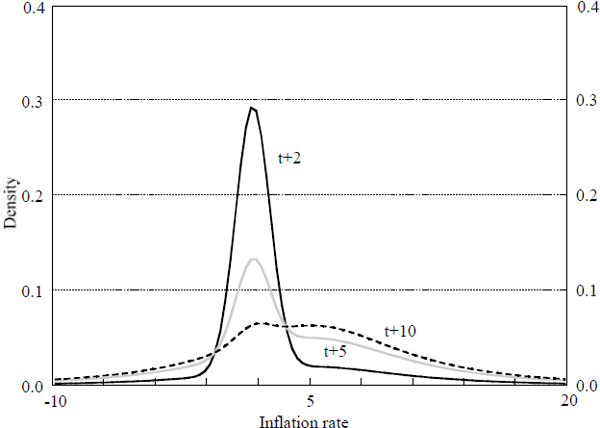
Figure 1 displays the probability densities of inflation under the current regime and under the assumption of a regime shift without any information on the inflation target in the new regime. Figure 2 displays the probability densities for inflation at different periods in the future. These densities are weighted averages of the two densities in Figure 1, with the weight on the regime-shift density increasing with the distance into the future. Clearly, the weighting of these two densities – each of which is symmetric – leads to a highly asymmetric density for future inflation over certain horizons.
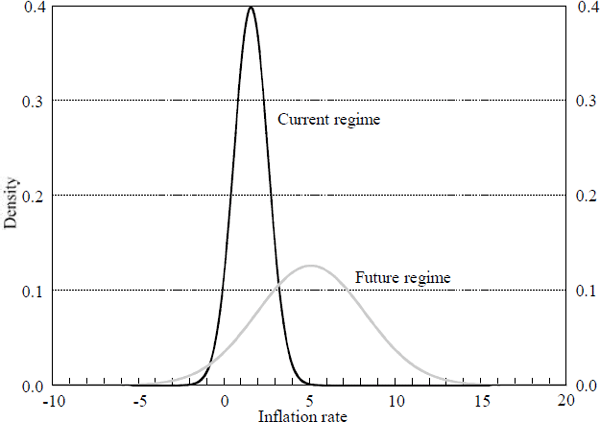
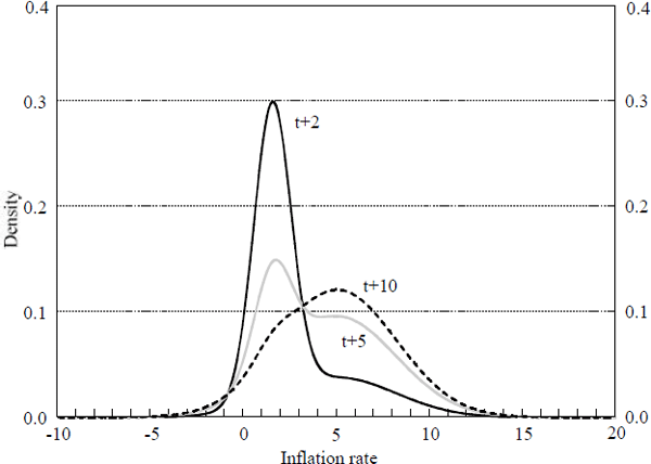
Table 1 displays the mean, median, and mode of inflation from 1 to 10 periods ahead. The asymmetry, as measured by the difference between the mean and the median, grows quickly and peaks in period t+3 before declining slowly over farther horizons. In period t+10 the density is quite close to the future regime density in Figure 1, which is symmetric. The density becomes bimodal in periods t+4 through t+9, with the second peak overtaking the first peak in period t+8. Over the entire 10-year period, the average of the mean inflation rates is 3.9 per cent, the average of the medians is 3.5 per cent, and the average of the modes is 2.7 per cent.
| Date | Mean | Median | Mode |
|---|---|---|---|
| t+1 | 1.5 | 1.5 | 1.5 |
| t+2 | 2.5 | 1.9 | 1.5 |
| t+3 | 3.3 | 2.4 | 1.6 |
| t+4 | 3.8 | 3.1 | 1.6 |
| t+5 | 4.2 | 3.6 | 1.7 |
| t+6 | 4.4 | 4.1 | 1.8 |
| t+7 | 4.6 | 4.5 | 2.0 |
| t+8 | 4.7 | 4.6 | 5.0 |
| t+9 | 4.8 | 4.7 | 5.0 |
| t+10 | 4.9 | 4.8 | 5.0 |
| Average | 3.9 | 3.5 | 2.7 |
3.2. Learning about the Current Regime
Of the four informational assumptions described at the beginning of the previous subsection, the most realistic are that agents know when there has been a regime change and that they know the probability of a regime change in any given period. Regime changes are likely to be associated with observable events such as a change in the party or individual in control of the central bank, an announcement by the central bank indicating that a new policy has been adopted, or a major economic or social shock such as a war. The probability of a regime change is given by the institutional structure of government and the randomness of individual career decisions and lifespans. It does not seem unreasonable to assume that agents understand this process well, or at least that their beliefs about it are not changing over time.
The first assumption that we relax is the assumption that agents know any new target inflation rate immediately. Instead, we assume that agents learn about the current regime by observing the inflation rates that occur. During the period in which a regime shift occurs, the best any agent can do is to expect future inflation to be equal to the mean across regimes, μ. (See Equation (9).) The probability density is given by the convolution of the target density and the density of deviations from target, shown in Equation (10).
In the following period, an inflation rate is observed. Assuming that there is no regime change, the optimal learning procedure is to use Bayes' rule to update the probability density of future inflation under the assumption that the current regime continues. The prior density is given by Equation (10). Equation (12) displays Bayes' rule, which uses the prior density combined with observed information on inflation in the current regime to determine the conditional probability density of future inflation under the assumption that the current regime survives. Since inflation one period ahead is not affected by any future regime change, its expected value is given by the standard formula for the expectation of a continuously distributed random variable displayed in Equation (11) using the density defined by Equation (12).
Once the current regime ends, the distribution of future inflation reverts to its prior distribution (Equation (10)). Thus, the probability density of inflation more than one period ahead takes the compound form presented in Equation (14). In all periods beyond t+2, the probability density of inflation is equal to the probability of no regime change times the density for period t+2 plus the probability of a regime change times the prior density of inflation under an unknown regime. The expected value of inflation in periods beyond t+2 (Equation (13)) takes a compound form parallel to Equation (14). Note that the expected value of inflation under the prior density is μ, the average inflation target across regimes.
After observing inflation in period t+2, the conditional density of inflation in period t+3 is given by Bayes' rule using the prior density (Equation (10)) and two pieces of information, πt+1 and πt+2. (This density is not shown.) As more periods of inflation are observed without a regime shift, the influence of the prior density diminishes and the conditional density of inflation approaches that of the case in which the current regime target inflation rate is known.
We now consider an example to illustrate the properties of this model. As in the previous section, suppose that the mean inflation target across regimes is 5 per cent with a standard deviation of 3 per cent, and that the probability of a new regime is 0.3 per period. Suppose that within a regime, the standard deviation of inflation around its target is 1 per cent, and that the current inflation target is 1.5 per cent. If a regime shift occurs in the current period, the conditional density of future inflation in every period is just given by the density under the assumption of a future regime shift as shown in Figure 1.
If a regime shift occurred last period and the regime survives in the current period, the distribution of next period's inflation depends on the current observation of inflation. Assuming that current inflation is 1.5 (the current inflation target) Figure 3 displays the probability density of inflation next period. For comparison, the density assuming complete knowledge of the current regime is also plotted. Note that the density with incomplete knowledge is more diffuse than that assuming complete knowledge. Figure 4 displays the probability densities for inflation at various periods in the future. These densities are weighted averages of the density in Figure 3 and the density assuming an unknown regime shift (shown in Figure 1). Once again, the weighting of these two densities – each of which is symmetric – leads to an asymmetric density for future inflation.
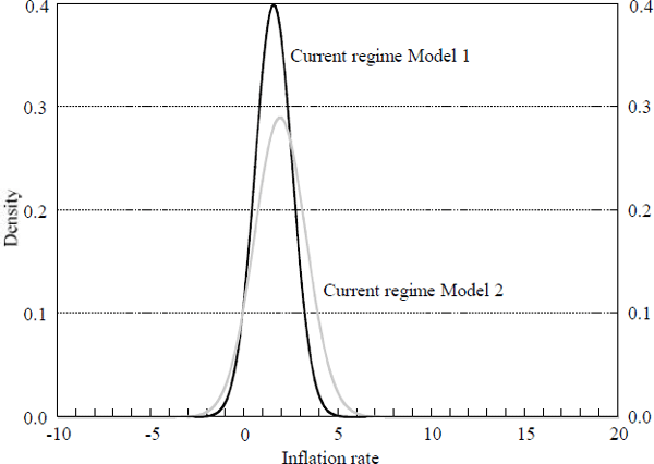
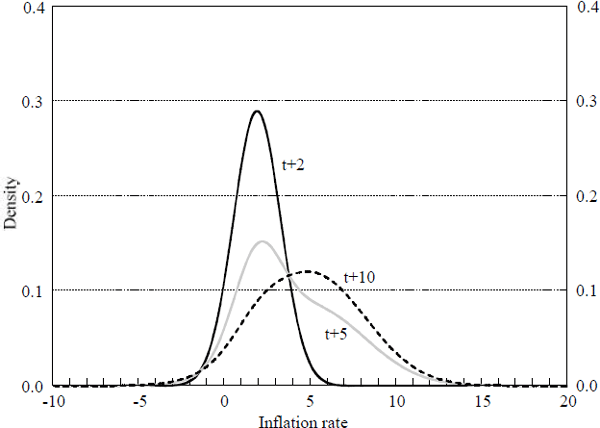
Table 2 displays the mean, median, and mode of inflation from 1 to 10 periods ahead, conditional on observing inflation in period t+1 after a regime shift in period t. The growing asymmetry is readily apparent, but not as extreme as in the case of complete knowledge of the current regime.
| Date | Mean | Median | Mode |
|---|---|---|---|
| t+1 | 1.8 | 1.8 | 1.8 |
| t+2 | 2.8 | 2.3 | 1.9 |
| t+3 | 3.5 | 2.8 | 2.0 |
| t+4 | 3.9 | 3.3 | 2.2 |
| t+5 | 4.2 | 3.8 | 2.4 |
| t+6 | 4.5 | 4.2 | 2.7 |
| t+7 | 4.6 | 4.4 | 3.6 |
| t+8 | 4.7 | 4.6 | 4.6 |
| t+9 | 4.8 | 4.7 | 4.8 |
| t+10 | 4.9 | 4.8 | 4.9 |
| Average | 4.0 | 3.7 | 3.1 |
3.3. Learning about Future Regimes
The other assumption that we relax is the assumption that agents know the distribution of target inflation rates across future regimes. In order to simplify the analysis we will return to the assumption that agents know the current and past inflation targets.
In this model, agents must estimate the mean and standard deviation of inflation targets across regimes using data on past regimes. Each time a new regime occurs, agents update their estimates of the mean and standard deviation. Expected inflation in the next period is simply the current inflation target, shown in Equation (15). Expected inflation more than one period ahead is a weighted average of the current inflation target and the average of current and past inflation targets (see Equation (16)). Since inflation regimes typically last for more than one period, the second term in Equation (16) is an average computed using the first year of each regime, denoted by the set {RN}, which contains N elements where N is the number of regimes. By the Law of Large Numbers, when N is large the right hand side of Equation (16) approaches equality with the right hand sides of Equations (2) and (3). In other words, when there have been many regimes in the past, agents can estimate the true mean of future inflation targets quite accurately.
The probability density of inflation one period ahead is given by Equation (17), which is identical to Equation (6). The probability densities of inflation more than one period ahead are given by Equation (18) under the assumption of a diffuse prior distribution on the mean and standard deviation of inflation targets across regimes. As the number of past regimes increases, this density approaches those of Equations (7) and (8), and we return to the case of complete knowledge about the distribution of future inflation targets,
To illustrate the properties of this model, we need to specify values of current and past inflation targets. To continue with the flavour of past examples, we choose past inflation targets of 4.5 and 9 per cent, and a current inflation target of 1.5 per cent. The average of these targets is 5 per cent and the standard deviation is 3 per cent. Thus, these outcomes are consistent with our earlier assumption of μ=5 and κ=3. Figure 5 displays the density of future inflation under the
assumption that there is a regime shift, i.e., the ratio of the triple integral to the double integral in Equation (18). For comparison, Figure 5 also displays the density of future inflation after a regime shift under the assumption of complete knowledge of the distribution of inflation targets, which was originally displayed in Figure 1. It is not surprising that the density without knowledge is more diffuse than the density with knowledge. Both densities are symmetric around the same mean, however, due to our choice of observed inflation targets with the same mean as the true distribution.
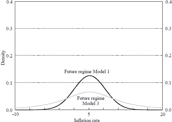
Figure 6 displays the densities of inflation in particular future periods. Once again, the densities are asymmetric whenever there is a positive probability that a regime shift may affect inflation in the period in question. Table 3 displays the mean, median, and mode of inflation in various future periods under the assumption that agents do not know the parameters of the distribution of future inflation targets and must infer them from observed inflation targets. The means and medians are identical to those displayed in Table 1 because the average of current and past inflation is assumed to be equal to the true mean of inflation targets across regimes. The only difference between Model 3 and Model 1 is that the density of inflation after a regime change is much more diffuse. This diffuseness affects the mode of future inflation since the secondary peak at 5 per cent inflation is much lower than in Model 1. This diffuseness has no effect on the mean or median of future inflation.
| Date | Mean | Median | Mode |
|---|---|---|---|
| t+1 | 1.5 | 1.5 | 1.5 |
| t+2 | 2.5 | 1.9 | 1.5 |
| t+3 | 3.3 | 2.4 | 1.5 |
| t+4 | 3.8 | 3.1 | 1.6 |
| t+5 | 4.2 | 3.6 | 1.7 |
| t+6 | 4.4 | 4.1 | 1.7 |
| t+7 | 4.6 | 4.4 | 1.7 |
| t+8 | 4.7 | 4.6 | 1.8 |
| t+9 | 4.8 | 4.7 | 4.9 |
| t+10 | 4.9 | 4.8 | 2.0 |
| Average | 3.9 | 3.5 | 1.6 |
Finally, we consider the effect of a new regime on the mean of future inflation in the case of learning about the distribution of inflation targets. Suppose that a new regime occurs in the example above with an inflation target of 1.5 per cent. In other words, suppose that a new central bank governor was installed who chose to continue the previous inflation target of 1.5 per cent. The effect of this new regime depends on the number of previously observed regimes. If there were only three previous regimes, the average of current and past inflation targets drops from 5 to 4.1 per cent. If there were ten previous regimes, which is the number of regimes estimated for Canada by RR, the average of current and past regimes declines by much less, from 5 to 4.7 per cent.
Footnotes
This property would not hold true if there were dependence across regimes. [5]
RR allow different serial correlation and variance of inflation in different regimes. In the high inflation regime they impose a unit root on the inflation rate which is not rejected by the data. With a unit root the population mean is undefined, but the sample mean is 9 per cent. [6]
RR allow different probabilities of a regime shift depending on the regime. For Canada, the probability of exiting a regime is close to 0.3 for each of the three regimes. [7]


