RDP 9810: The Distribution and Measurement of Inflation Appendix C: Example of the Calculation of Trimmed Means
September 1998
- Download the Paper 326KB
This appendix briefly describes the calculation of trimmed means, and in particular the 100 per cent trimmed mean, and gives a simple example of their construction in Table C2 using data in Table C1. All series use the time-varying weights as defined in Appendix A.
| Component | A | B | C | D | E | F |
|---|---|---|---|---|---|---|
| Price change (per cent) | −1.00 | 0.00 | 0.30 | 0.80 | 0.90 | 2.00 |
| Time-varying weight | 0.10 | 0.15 | 0.20 | 0.25 | 0.15 | 0.15 |
| Cumulative weight | 0.10 | 0.25 | 0.45 | 0.70 | 0.85 | 1.00 |
| Weight for 50 per cent trim | 0.00 | 0.00 | 0.40 | 0.50 | 0.10 | 0.00 |
| Measure | Calculation | Result |
|---|---|---|
| Mean | (0.1×−1)+(0.15×0)+(0.2×0.3)+(0.25×0.8)+ (0.15×0.9)+(0.15×2) |
0.60 |
| 50 per cent trimmed mean | (0.4×0.3)+(0.5×0.8)+(0.1×0.9) | 0.61 |
| Median – used in this paper | price change of component D | 0.80 |
| Median – alternative definition | 0.45+(0.8−0.3) × (0.50−0.45)/(0.70−0.45) | 0.63 |
The X per cent trimmed mean removes X per cent of the components of the CPI basket whose price changes lie in the tails of the cross-sectional distribution of price changes. For example, the symmetric 50 per cent trimmed mean removes both the 25 per cent of the basket with the largest and smallest price changes. An asymmetric trimmed mean will remove a different proportion from the left- and right-hand tails. A component that lies partially in the tail removed, has its weight reduced proportionately. The weights of the remaining components are then scaled to sum to unity, with the trimmed mean calculated as the sum of the products of the component inflation rates and scaled weights.
The median, or 100 per cent trim, in this paper, as in Shiratsuka (1997) is calculated as the price change of the component covering the 50th percentile. If the 100 per cent trim is asymmetric, it is the price change of the component covering the percentile on which the trimmed mean is centred. For example, if 53 per cent of a 100 per cent trim is taken from the left tail, it will be the price change of the component covering the 53rd percentile.
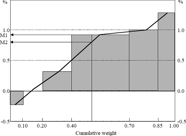
Alternatively, the median can be calculated as a weighted average of the component covering the 50th percentile and the adjacent component as in Laflèche (1997). This method seeks to make the discrete distribution of price changes continuous. Laflèche (1997) joins the components through the upper percentile of each component. Since the price change for each CPI component is the average price change for all goods and services in that component, the distribution should be joined through the middle percentile of each component, as in Figure C1. This method can also be applied to asymmetric 100 per cent trimmed means or smaller trimmed means. The price change of a given component is used as the 100 per cent trimmed mean in this paper, as it is less complex and so more intuitive. Because the CPI data used in this study are highly disaggregated, and price changes are tightly clumped at the centre of the distribution, the two methods of calculating the median produce almost identical results. From December 1980 to March 1998, the MAD between the medians based on the alternative definitions is 0.0001 of a percentage point.

Note: M1 is the median as calculated in this paper, M2 is the alternative definition of the median.