RDP 2000-07: The Effect of Uncertainty on Monetary Policy: How Good are the Brakes? 3. Uncertainty and Smoothing
October 2000
- Download the Paper 278KB
The long-standing explanation for the observed smoothness of policy interest rates is that policy decisions are made under uncertainty. Until recently, this had rarely been taken into account explicitly in policy models, as additive (mean-zero) shocks were generally the only form of uncertainty considered. As most models assumed a quadratic objective function for policy (most commonly, squared deviations of inflation from target and output from potential), the economy was linear and its structure known to the policy-maker, then certainty equivalence implied that the policy-maker's uncertainty about the future shocks would not affect the policy decision.
More recently, Brainard's (1967) discussion of uncertainty has been seriously reconsidered. Brainard noted that while certainty equivalence implies that additive uncertainty provides no justification for smooth adjustment of policy, multiplicative uncertainty can. In this section, we discuss four aspects of multiplicative uncertainty – model uncertainty, parameter uncertainty, mean parameter uncertainty and data uncertainty – and their impact on policy outcomes. The first of these encompasses the latter three but the distinction is useful for expository purposes.
3.1 Model uncertainty
At the most general level, the policy-maker may be uncertain about the model that best describes the economy. Parameter uncertainty is a particular form of this, where only uncertainty about the variables included in a particular model is considered. Model uncertainty takes into account the possibility that omitted variables in a model may actually have non-zero coefficients.
Blinder (1995a) provides a simple solution to the dilemma of model uncertainty: ‘use a wide variety of models and don't ever trust any one of them too much.’ Sargent (1999) and Onatski and Stock (2000) address Blinder's solution more technically and find that such uncertainty generally results in a more aggressive approach as the policy-maker seeks to avoid ‘worst-case’ outcomes.
Both of these latter analyses address the issue of ‘robust’ control across a range of possible models of the economy rather than ‘optimal’ control within one particular model. Sargent describes the policy-maker's decision process in such a world as ‘planning against [the worst, thereby] assuring acceptable performance under a range of specification errors’ (p 5). That is, the policy-maker practises disaster avoidance. Whether this cautious approach implies more or less aggressive policy actions, Sargent argues, depends on the nature of the disasters to be avoided. Of relevance to the results obtained below, Onatski and Stock find that the possibility that monetary policy might have almost no effect prompts a more aggressive response.
A similar consideration of robust control in the context of monetary policy rules has long been advocated by McCallum.[6] He argues that the robustness of a monetary policy rule across different economic models is a crucial characteristic in determining a rule that the central bank should follow. However, robustness of this sort has generally been examined in an environment of additive uncertainty only, where no account has been taken of the parameter uncertainty within each model (see, most notably, the volume edited by Bryant, Hooper and Mann (1993)).
3.2 Parameter uncertainty
In his analysis, Brainard focused explicitly on uncertainty about the parameters in the model that describes the economy. In particular, there may be uncertainty about the impact of interest changes on output and inflation. In this environment, the policy-maker has to trade off the desire to return these variables to their target values as quickly as possible, with the desire to minimise the risk of increased volatility in output and inflation that arise because policy changes might have a larger (or smaller) impact than expected. As a consequence, in the one-period model that Brainard uses, the policy-maker moves interest rates by less to return inflation and output to target than if there were no uncertainty.
The presence of parameter uncertainty does not necessarily imply that the policy-maker should be less aggressive (i.e., produce a path of policy rates that is smoother), particularly when there is uncertainty about more than one parameter. Whether or not it does, is essentially an empirical question. Using a model of the Australian economy, Shuetrim and Thompson (1999) find that uncertainty about the economy's dynamics can increase or reduce the activism of policy, depending on the location of the uncertainty. In the US context, Wieland (1998) also argues that uncertainty-induced caution does not allow the policy-maker the benefit of experimentation to better learn the true structure of the economy. In a non-linear world, however, such experimentation may be particularly costly.
In contrast, Sack (2000) finds that the introduction of parameter uncertainty to a VAR model of the US economy reconciles much of the difference between the observed path of the Fed funds rate and that implied by a VAR model without such uncertainty. Martin and Salmon (1999) replicate these results for the UK. In each case, however, as the aim of the exercise was to reconcile the estimated path of policy interest rates and the path that actually occurred, while parameter uncertainty was taken into account, only the observed path of additive shocks was considered.
3.3 Mean parameter uncertainty
Another particular form of model uncertainty is mean parameter uncertainty (Rudebusch 1999). The form of parameter uncertainty described in the previous section assumes that, for example, the effect of interest rates on activity is (normally) distributed about the mean estimated within the model. Thus there is only a small possibility that interest rates will have an impact that is surprisingly large. In practice, however, the policy-maker may believe that the average impact of interest changes is considerably larger (or smaller) than that implied by the model, perhaps because the model is mis-specified.
In a deterministic world, the greater the average impact of policy changes on the economy the less aggressive will those policy changes be. If there is also parameter uncertainty, the result is not so clear cut. This is most easily seen in the following variant of the Svensson (1997) model discussed by Batini, Martin and Salmon (1999):
where y is output, i, the policy interest rate and π is inflation.
If inflation is the sole objective for monetary policy and the target rate of inflation is zero, the optimal interest rate is given by
where  and
and
 are the
means of the parameters in the two equations, and
  is the variance
of b.
In this model, whether an increase in average interest sensitivity (an increase in  ) increases
or decreases the aggressiveness of monetary policy depends on whether the coefficient of
variation
  (the inverse of the t-statistic) is greater than or less than one. If the interest rate
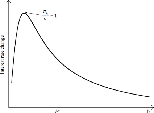
term is statistically significant (b* in Figure 2), the coefficient of
variation is less than one, and hence, an increase in interest sensitivity (an increase in
b) decreases the aggressiveness of monetary policy.

Conversely, if we decrease the interest sensitivity parameter (while maintaining the same degree of uncertainty about it), initially this will increase the aggressiveness of monetary policy. However, once the mean of the parameter is less than one standard deviation from zero, further declines in it will actually decrease policy aggressiveness. This is because the costs of ‘perverse’ outcomes, whereby an increase in interest rates leads to an increase in inflation, are large enough to offset the benefits of the ‘normal’ case of an increase in interest rates leading to a decrease in inflation. These arguments are illustrated in Figure 2, which plots the interest rate change necessary to return inflation to target in the event of a deviation from target, as the mean value of the interest rate sensitivity parameter, b, is changed.
Table 2 summarises the effect of a sustained 50 basis point change in policy rates as estimated in representative macroeconomic models in the US, the UK and Australia. The individual impact of any one change is not particularly large, given the intense attention that accompanies any policy change. This suggests that the general public and financial markets, as well as perhaps policy-makers, may believe that the effect is indeed larger than empirically estimated. Alternatively, it may support the argument of Woodford (1999) discussed above, that a change in policy generates expectations of more changes in the same direction in the future.
The existing empirical work has generally not addressed this form of mean parameter uncertainty. Rudebusch (1999) finds that uncertainty about the average interest sensitivity of output or about the persistence of inflation has some impact on the aggressiveness of policy, but that mean uncertainty about the slope of the Phillips curve or output persistence has little impact.
| After 4 quarters | After 8 quarters | |
|---|---|---|
| Australia | ||
| GDP Growth | 0.26 | 0.35 |
| Inflation | 0.18 | 0.33 |
| US | ||
| GDP Growth | 0.3 | 0.55 |
| Inflation | 0.1 | 0.3 |
| UK | ||
| GDP Growth | 0.23 | 0.53 |
| Inflation | 0.13 | 0.51 |
|
Sources: Australia: Beechey et al (2000) |
||
3.4 Data uncertainty
Finally, the possibility of data revisions may imply that the policy-maker is uncertain about the current economic situation. In the absence of other uncertainty, data revisions are just another source of additive uncertainty, and hence, certainty equivalence implies that they should have no impact on the policy decision. Thus, the inclusion of data uncertainty will not affect the optimal policy benchmark. However, if Taylor rules are used as the benchmark for policy, data revisions will play a role, because certainty equivalence no longer applies (Orphanides 1998).
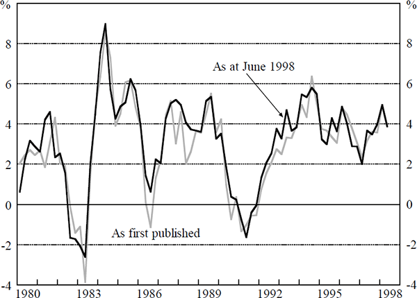
In Australia, as in most countries, one important source of data uncertainty is revisions to GDP. Figure 3 shows the divergence between the first published estimate of four-quarter-ended GDP growth and the current estimate.[7] If one were to compare the first published estimate of the level of GDP with the most recent estimate, the divergence would be even greater, as, in Australia, revisions to GDP are, on average, upwards.

For the policy-maker and for policy models that incorporate a Phillips-curve type supply-side, this poses particular problems for the estimate of the output gap. Estimating potential output is problematic even in the absence of revisions to the estimate of actual GDP. Orphanides (1998) shows that introducing real-time output gap uncertainty into a model of US monetary policy, results in a policy that is considerably less aggressive than that implied by a policy rule that ignores such considerations. Rudebusch (1999) finds that data uncertainty reduces the aggressiveness of policy to deviations of inflation and output from target in a Taylor rule. More fundamentally, Isard, Laxton and Eliasson (1999) consider the performance of various monetary policy rules in a non-linear model of the US economy with uncertainty about the output gap and find that Taylor-type rules are generally not robust.

