RDP 2001-03: The Response of Financial Markets in Australia and New Zealand to News About the Asian Crisis 4. Comparing Spillover in Crises and at Other Times
July 2001
- Download the Paper 677KB
An important question relating to financial stability is whether the spillover of shocks and volatility is greater when the originating markets are in crisis, than in more-normal times. At first glance, it might be thought that this is true: turbulent markets indicate greater uncertainty about the future, and so uncertainty about the effects of news events on third markets is also likely to be greater during these times.
It is not feasible to answer this question using the news-event data described in Section 2.3, however. By construction, there were no news events before or after the Asian crisis period (May 1997–August 1998), so we cannot test whether markets responded more to news events in the Asian crisis period than in other periods. Instead, we estimate an expanded version of the VARs presented in Section 3.2, with an additional equation in the system to measure movements in Asian financial markets. We present results for returns, rather than volatility (absolute returns), as these were more robust to small specification changes, and allow us to examine the direction as well as magnitude of the reaction to movements in other markets.
For each market, we present selected impulse responses and variance decompositions, using a recursive-ordering identification scheme with the ordering {Asia, Australia, New Zealand, US}. In general, alternative orderings made little difference to our results on the effect of the Asian variable on returns in Australia and New Zealand, although the relative ordering of Australia and New Zealand can affect the estimates of their effects on each other. The US market generally had no contemporaneous effect on the Australian and New Zealand markets, even when the system was ordered to permit this. We attribute this result to the time-zone differences, with the US trading day starting after the close in Asian, Australian and New Zealand markets.
To capture movements in Asian financial markets, we use regional indices. For stock markets, we use the MSCI Far East Free (excluding Japan) Index compiled by Morgan Stanley. This index is a market-capitalisation weighted stock price index covering at least 60 per cent of the market capitalisation of each industry group. Only the portion of each country's stock market that is freely available to overseas investors is included. We use these ‘Free’ series on the basis that contagion reflects movements in markets that foreigners can invest in, rather than those which only domestic investors can access. The countries included are listed in column 1 of Table 8, the data are presented in Figure 6.[11] Although we have elected to use a series that incorporates countries other than those most affected by the crisis (i.e. Indonesia, Korea, Thailand, Malaysia and the Philippines), this does not appear to distort our results. We obtained very similar results for the impulse responses and variance decompositions using the MSCI Emerging Markets Far East Index, the MSCI Emerging Markets Asia Index, and the first principal component of a data set of stock-market returns for the five countries most affected by the Asian crisis.[12]
| MSCI Far East Free (excl Japan) |
MSCI Emerging Markets Far East |
MSCI Emerging Markets Asia |
EMBI Global Constrained (Asia sub-index) | Troubled Asian exchange rate index |
|---|---|---|---|---|
| China | China | China | China | |
| Hong Kong | ||||
| India | ||||
| Indonesia | Indonesia | Indonesia | Indonesia (JCI) | |
| Korea | Korea | Korea | Korea | Korea (KOSPI) |
| Malaysia | Malaysia | Malaysia | Malaysia | Malaysia (KLCI) |
| Pakistan | ||||
| Philippines | Philippines | Philippines | Philippines | |
| Singapore | ||||
| Sri Lanka | ||||
| Taiwan | Taiwan | Taiwan | ||
| Thailand | Thailand | Thailand | Thailand | Thailand (SET) |
|
Sources: MSCI indices: Morgan Stanley and Bloomberg. EMBI Global: JP Morgan. Exchange-rate index compiled by the authors. |
||||
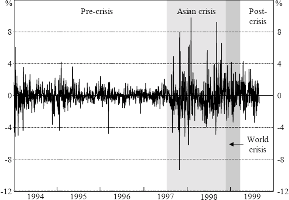
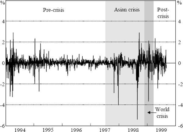
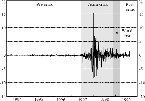
Analysis of an equivalent VAR system for bond returns is precluded by the lack of long-maturity sovereign debt securities in the crisis-affected countries, equivalent to the benchmark bonds used for Australia, New Zealand and the United States. Instead, we use the JP Morgan EMBI (Emerging Markets Bond Index) Global Constrained Asia sub-index series as a proxy (Figure 7). This series is constructed using USD-denominated eurobonds for countries without a well-developed own-market for sovereign debt.[13] For the exchange rate, we constructed a GDP-weighted fixed-weight exchange-rate index based on the spot exchange rates of the four countries listed in the right-most column of Table 8 against the USD (Figure 8). The GDP weights were based on 1996 data from the World Bank Atlas (1998), which converts the local-currency GDP levels to USD using three-year-average exchange rates. A fall in this index represents depreciations of these countries' currencies against the USD.
One rationale for using a regional index is that it summarises groups of explanators that are not of interest individually. With multiple individual series (plus lags) in the system, estimated coefficients for the crisis periods compared with non-crisis periods could be higher for some series and lower for others. In that case, it is not clear whether ‘spillover’ in a general sense is greater or smaller during periods of financial crisis. By summarising the data using a regional index (or a principal component), we can get a better sense of the net difference between crisis periods and non-crisis periods.
Furthermore, and not surprisingly, the returns in individual Asian countries are correlated (individual daily stock market returns have correlation coefficients as high as 0.36). We are less interested in identifying the separate effects of movements in each market, than in determining the reaction in Australia and New Zealand to some broadly defined notion of movements in Asian markets. Using the regional index instead of the country-specific data allows us to capture movements in Asian financial markets, while avoiding the problems inherent in estimating systems with multicollinear explanators.
Another consideration that suggests some sort of data-summary technique may be more appropriate is the loss of observations due to public holidays and other non-trading days falling on different days in different countries. For the VARs presented in Section 3.2 above, there is enough overlap between non-trading days in the different countries so that the number of observations lost is small. However, when Asian markets are added, around half the total number of observations can be lost due to missing data on non-trading days. This wastage of data points is clearly undesirable. By contrast, the regional indices record price movements for days when some (but not all) of those markets are closed, although possibly at the expense of some measurement error.
4.1 Stock Markets
Within each sub-period (pre-crisis, Asian crisis, world crisis, and post-crisis), our VAR results for stock returns were largely as expected. Much of the variation in Australian and New Zealand returns was driven by overnight developments in US markets. Movements in the Australian and New Zealand markets did not have an independent effect on US markets. There was some minor persistence in Australasian markets, with lagged own-price changes being significant in some cases. The previous day's return in the Australian market also had a significant positive effect on the New Zealand market; we attribute this to time-zone differences.[14]
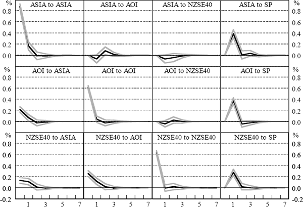
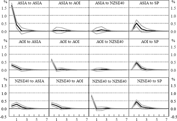
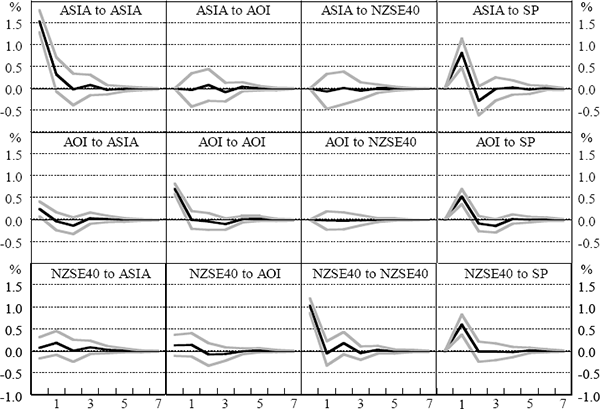
The impulse responses shown in Figures 9–12, and the variance decompositions in Tables 9–12, are based on the recursive identification scheme discussed above, that is, {Asia, Australia, New Zealand, US}. We cannot be sure that we have identified true structural innovations using this scheme. However, we are confident that a different ordering within a recursive scheme would not appreciably affect the results. The impulse responses and variance decompositions derived using other possible orderings are very similar to those presented here.[15] In particular, even when the US variable (S&P500) was ordered before the other variables, allowing it to affect all other variables contemporaneously, the impulse responses of the other variables to an innovation in the S&P500 were still tent-shaped, with the contemporaneous responses being close to (and almost always insignificantly different from) zero. A similar result applied for the bond and foreign exchange market results presented in the following sections.

| Period | SE | ASIA | AOI | NZSE40 | S&P500 |
|---|---|---|---|---|---|
| Asia: MSCI Far East Free excluding Japan | |||||
| 0 | 0.879 | 100.00 | 0.00 | 0.00 | 0.00 |
| 1 | 0.981 | 83.29 | 0.43 | 0.44 | 15.84 |
| 4 | 0.986 | 82.42 | 1.15 | 0.62 | 15.81 |
| All Ordinaries Index | |||||
| 0 | 0.652 | 11.22 | 88.78 | 0.00 | 0.00 |
| 1 | 0.757 | 9.23 | 66.21 | 0.27 | 24.29 |
| 4 | 0.760 | 9.27 | 65.82 | 0.40 | 24.51 |
| NZSE40 | |||||
| 0 | 0.698 | 3.73 | 13.81 | 82.47 | 0.00 |
| 1 | 0.770 | 5.20 | 13.71 | 67.81 | 13.28 |
| 4 | 0.771 | 5.22 | 13.75 | 67.70 | 13.33 |
| S&P500 | |||||
| 0 | 0.653 | 0.71 | 0.48 | 0.19 | 98.63 |
| 1 | 0.657 | 0.75 | 0.66 | 0.34 | 98.26 |
| 4 | 0.658 | 0.79 | 0.66 | 0.37 | 98.18 |
|
Note: The second through fifth data columns of the table represent the percentage of error variance in the current period accounted for by current-period innovations to each variable in the model; these four columns should therefore sum to 100. |
|||||
| Period | SE | ASIA | AOI | NZSE40 | S&P500 |
|---|---|---|---|---|---|
| Asia: MSCI Far East Free excluding Japan | |||||
| 0 | 1.663 | 100.00 | 0.00 | 0.00 | 0.00 |
| 1 | 1.789 | 91.58 | 0.10 | 0.01 | 8.30 |
| 4 | 1.799 | 90.55 | 0.22 | 0.31 | 8.92 |
| All Ordinaries Index | |||||
| 0 | 0.719 | 18.65 | 81.35 | 0.00 | 0.00 |
| 1 | 0.874 | 16.28 | 55.16 | 0.01 | 28.56 |
| 4 | 0.884 | 15.96 | 54.23 | 0.24 | 29.57 |
| NZSE40 | |||||
| 0 | 0.883 | 3.58 | 11.57 | 84.85 | 0.00 |
| 1 | 1.049 | 9.99 | 11.60 | 60.09 | 18.33 |
| 4 | 1.066 | 10.74 | 11.48 | 58.34 | 19.43 |
| S&P500 | |||||
| 0 | 1.086 | 6.50 | 0.33 | 1.46 | 91.71 |
| 1 | 1.092 | 6.66 | 0.49 | 1.56 | 91.29 |
| 4 | 1.086 | 6.50 | 0.33 | 1.46 | 91.71 |
| Note: See Table 9 | |||||
| Period | SE | ASIA | AOI | NZSE40 | S&P500 |
|---|---|---|---|---|---|
| Asia: MSCI Far East Free excluding Japan | |||||
| 0 | 1.535 | 100.00 | 0.00 | 0.00 | 0.00 |
| 1 | 1.769 | 78.68 | 0.03 | 0.13 | 21.16 |
| 4 | 1.798 | 76.42 | 0.49 | 0.21 | 22.88 |
| All Ordinaries Index | |||||
| 0 | 0.751 | 10.94 | 89.06 | 0.00 | 0.00 |
| 1 | 0.920 | 7.41 | 59.32 | 0.03 | 33.25 |
| 4 | 0.951 | 9.13 | 56.75 | 0.10 | 34.03 |
| NZSE40 | |||||
| 0 | 1.046 | 0.53 | 1.63 | 97.85 | 0.00 |
| 1 | 1.232 | 2.76 | 2.52 | 70.71 | 24.00 |
| 4 | 1.254 | 3.21 | 3.06 | 70.52 | 23.22 |
| S&P500 | |||||
| 0 | 1.390 | 1.73 | 4.24 | 0.00 | 94.02 |
| 1 | 1.408 | 1.72 | 5.48 | 0.36 | 92.44 |
| 4 | 1.444 | 2.81 | 7.48 | 0.55 | 89.17 |
|
Note: See Table 9 |
|||||
| Period | SE | ASIA | AOI | NZSE40 | S&P500 |
|---|---|---|---|---|---|
| Asia: MSCI Far East Free excluding Japan | |||||
| 0 | 1.255 | 100.00 | 0.00 | 0.00 | 0.00 |
| 1 | 1.450 | 80.51 | 0.14 | 0.20 | 19.15 |
| 4 | 1.473 | 78.52 | 0.19 | 2.51 | 18.79 |
| All Ordinaries Index | |||||
| 0 | 0.621 | 14.28 | 85.72 | 0.00 | 0.00 |
| 1 | 0.767 | 9.49 | 56.85 | 0.48 | 33.18 |
| 4 | 0.774 | 10.19 | 56.01 | 0.52 | 33.28 |
| NZSE40 | |||||
| 0 | 0.808 | 7.04 | 6.73 | 86.22 | 0.00 |
| 1 | 0.912 | 5.69 | 7.03 | 68.25 | 19.03 |
| 4 | 0.937 | 5.71 | 7.43 | 67.55 | 19.31 |
| S&P500 | |||||
| 0 | 1.147 | 0.01 | 0.07 | 0.35 | 99.57 |
| 1 | 1.158 | 0.18 | 0.09 | 2.04 | 97.69 |
| 4 | 1.168 | 0.77 | 0.30 | 2.05 | 96.87 |
| Note: See Table 9 | |||||
The variance decompositions for the four periods show that own-market innovations are the most important, although the S&P500 has a significant impact on the Australian and New Zealand indices in all periods. The effect of the Asian market variable on Australian and New Zealand stocks was also fairly important, particularly during the Asian crisis period. There was some apparent cross-determination between the Australian and New Zealand markets, although this was not robust to different relative orderings. As expected, the S&P500 was virtually entirely driven by own-market innovations, although the contribution of the Asian variable in the crisis period was higher than at other times.[16]
When we examine each of the sub-periods individually, however, we obtain results that conflict with the usual intuition about the spillover of financial-market volatility, i.e. that transmission of volatility from one market to another should be greater in times of crisis than in more-normal times. The implied response of Australian and New Zealand stocks to an innovation from the Asian series was proportionately smaller in both the Asian and world crisis periods than in the pre-crisis period. The impulse response peaked at around 0.2–0.3 percentage points in both the pre-crisis and Asian crisis periods, even though the size of a one-standard-deviation innovation in the Asian series was twice as large in the Asian crisis period as in the pre-crisis period. Moreover, the reaction in the post-crisis period was similar to the reaction in the Asian crisis, and greater than in the world crisis period.
4.2 Bond Markets
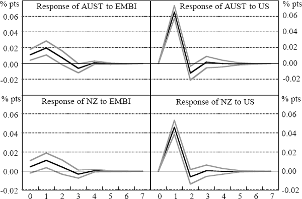
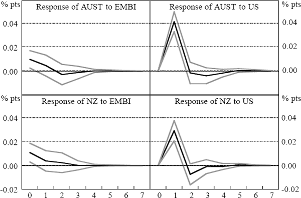
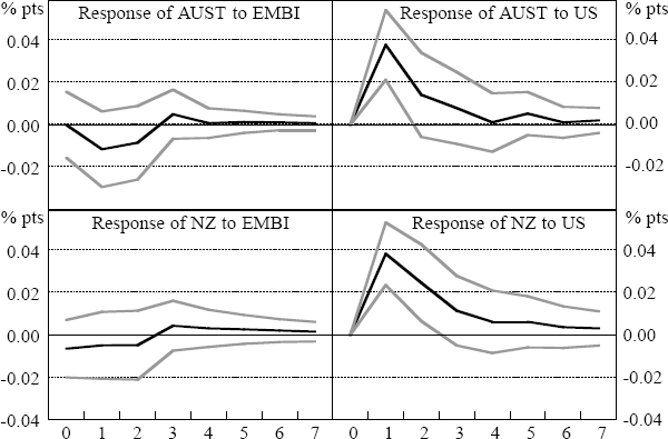
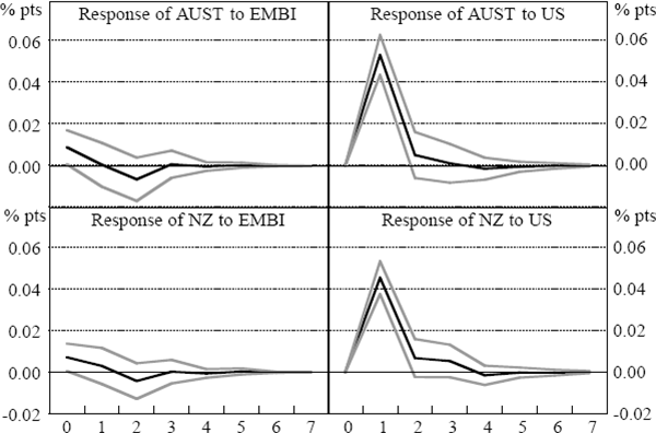
Figure 14 suggests that returns on the EMBI Global Constrained Index had a small and marginally significant impact on Australian and New Zealand bond returns during the Asian crisis period. However, the greatest reaction of Australian and New Zealand bond returns to the Asian series was in the pre-crisis period (Figure 13).[17] This result may be due to the EMBI series picking up the effects of the Japanese and European markets on Australian and New Zealand bond yields. Previous work has suggested some role for these other markets, independent of the US market, in explaining bond-market movements in Australia (Kortian and O'Regan 1996). Since these markets are omitted from our estimates, it may be that the EMBI series is picking up innovations from those markets during the 1994 bond market sell-off. If the Japanese and European market had affected Asian markets as well as the Australian and New Zealand markets, then our identification approach will capture this as Australian and New Zealand returns being affected by Asian returns.
| Period | SE | AUST | NZ | US | EMBI |
|---|---|---|---|---|---|
| Australian bond futures | |||||
| 0 | 0.085 | 98.22 | 0.00 | 0.00 | 1.78 |
| 1 | 0.110 | 59.73 | 0.23 | 35.65 | 4.39 |
| 4 | 0.111 | 58.57 | 0.30 | 36.10 | 5.03 |
| New Zealand bond futures | |||||
| 0 | 0.081 | 18.27 | 81.40 | 0.00 | 0.33 |
| 1 | 0.095 | 13.60 | 60.79 | 23.90 | 1.70 |
| 4 | 0.095 | 13.52 | 60.37 | 24.11 | 2.00 |
|
Note: See Table 9 |
|||||
| Period | SE | AUST | NZ | US | EMBI |
|---|---|---|---|---|---|
| Australian bond futures | |||||
| 0 | 0.062 | 97.53 | 0.00 | 0.00 | 2.47 |
| 1 | 0.075 | 67.29 | 0.38 | 30.26 | 2.07 |
| 4 | 0.076 | 67.09 | 0.41 | 30.27 | 2.23 |
| New Zealand bond futures | |||||
| 0 | 0.067 | 15.32 | 82.05 | 0.00 | 2.63 |
| 1 | 0.073 | 12.83 | 68.87 | 15.83 | 2.47 |
| 4 | 0.074 | 12.76 | 68.04 | 16.66 | 2.54 |
Note: See Table 9 |
|||||
There does not appear to be an indirect response to Asia via the US market. Overnight developments in US bond markets had a strong effect on Australian and New Zealand bond returns, accounting for 15–30 per cent of their variability in the Asian crisis period, around 40 per cent in the world crisis and around 66 per cent in the post-crisis period at the one to four-day horizon. However, during the Asian crisis (and the world crisis), bond market volatility in Asia, as proxied by EMBI, accounted for an insignificant part of the variation in the US market (less than one per cent).[18]
There are a number of possible reasons for this smaller response to Asian crisis events by bonds than for stocks. In particular, bond yields are determined primarily by expectations of inflation and (domestic) real interest rates. Therefore, bond returns should be less affected by corporate sector and trade developments than are other markets, and so the economic-linkages rationale for contagion between asset markets (Lowell et al 1998) is not as important. This would tend to result in a more muted reaction in bond markets than for stocks and, particularly, exchange rates.
| Period | SE | AUST | NZ | US | EMBI |
|---|---|---|---|---|---|
| Australian bond futures | |||||
| 0 | 0.065 | 100.00 | 0.00 | 0.00 | 0.00 |
| 1 | 0.079 | 74.59 | 0.28 | 23.02 | 2.12 |
| 4 | 0.081 | 70.27 | 0.51 | 25.75 | 3.47 |
| New Zealand bond futures | |||||
| 0 | 0.057 | 34.44 | 64.27 | 0.00 | 1.29 |
| 1 | 0.069 | 23.40 | 44.42 | 30.82 | 1.36 |
| 4 | 0.075 | 20.24 | 37.72 | 39.96 | 2.08 |
| Note: See Table 9 | |||||
| Period | SE | AUST | NZ | US | EMBI |
|---|---|---|---|---|---|
| Australian bond futures | |||||
| 0 | 0.050 | 99.16 | 0.00 | 0.00 | 0.84 |
| 1 | 0.090 | 31.04 | 0.84 | 67.55 | 0.57 |
| 4 | 0.092 | 30.10 | 2.33 | 66.23 | 1.34 |
| New Zealand bond futures | |||||
| 0 | 0.039 | 33.55 | 66.45 | 0.00 | 0.00 |
| 1 | 0.070 | 10.41 | 21.72 | 67.36 | 0.51 |
| 4 | 0.071 | 10.30 | 22.31 | 65.31 | 2.08 |
|
Note: See Table 9 |
|||||
4.3 Exchange Rates
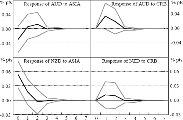
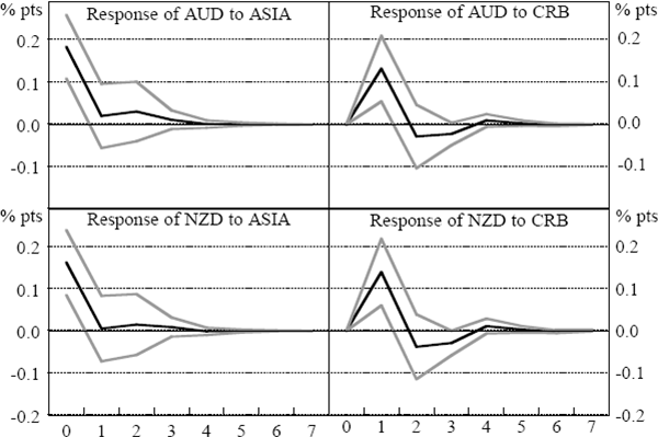
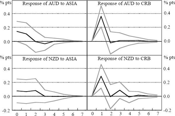
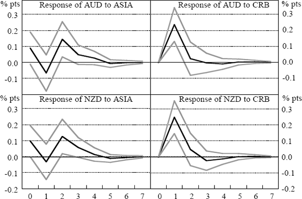
There was a clear reaction of the AUD/USD and NZD/USD to movements in Asian markets during the Asian crisis (Figure 18). This response was much more obvious than in the other two markets. Exchange-market movements in Asia were significant during the Asian crisis, accounting for just under 8 per cent of the variation in the AUD/USD rate, and around 5½ per cent of the NZD/USD at each of the horizons examined (Table 18).[19] There was also a significant impact on the NZD/USD rate in the pre-crisis period (Table 17). In the other periods, the impulse responses were not more than two standard deviations from zero (although nearly so for the AUD/USD in the world crisis). While this might partly reflect the poor fit of the linear model – evidenced by the large error bands in most periods – it makes the contrast with the Asian crisis period even more striking.
As might be expected from the results in Section 3.2, another feature of these results is the increasing importance over time of the CRB index in explaining daily movements in both the AUD/USD and NZD/USD exchange rates. This is demonstrated in the increasing share of total variance accounted for by the CRB index in a sequential comparison of the variance decompositions reported in Tables 17–20. Since Australia and New Zealand's exports have tended to become more diverse over time, rather than more concentrated in commodities, this result cannot reflect changing fundamentals. In any case, the extent of the change in exchange-rate behaviour is probably too dramatic to be explained by a shift in the composition of exports. Moreover, the composition of the CRB index is not a particularly good match with the commodities exported by Australia and New Zealand, perhaps suggesting that short-term movements in these exchange rates have become less aligned with genuine fundamentals over time. This type of development may be evidence that financial market integration brings an increased proportion of less-informed traders to regional markets, who may look to indicator variables with little information content – but high-frequency availability – in forming their views and trading strategies. In this context, the theoretical findings of Calvo and Mendoza (1999) seem particularly pertinent. On the other hand, the increasing importance of the CRB index may simply reflect that the shocks to commodity prices were concentrated in the components of the index most relevant to Australian and New Zealand exports, despite the index as a whole being an imperfect measure of prices of these exports. Similarly, it may have been that all types of commodity prices responded to changing prospects for world growth in the world crisis and post-crisis period. Therefore the CRB index might have been more correlated with these exchange rates in those periods despite the differences between the composition of the CRB index and Australian and New Zealand exports.
| Period | SE | AUD | NZD | CRB | ASIA |
|---|---|---|---|---|---|
| AUD/USD | |||||
| 0 | 0.468 | 99.60 | 0.00 | 0.00 | 0.40 |
| 1 | 0.469 | 99.03 | 0.01 | 0.56 | 0.41 |
| 4 | 0.470 | 98.60 | 0.18 | 0.74 | 0.48 |
| NZD/USD | |||||
| 0 | 0.360 | 21.98 | 75.80 | 0.00 | 2.22 |
| 1 | 0.361 | 22.21 | 75.27 | 0.10 | 2.43 |
| 4 | 0.363 | 22.13 | 75.29 | 0.17 | 2.41 |
| Note: See Table 9 | |||||
| Period | SE | AUD | NZD | CRB | ASIA |
|---|---|---|---|---|---|
| AUD/USD | |||||
| 0 | 0.660 | 92.23 | 0.00 | 0.00 | 7.77 |
| 1 | 0.673 | 88.59 | 0.00 | 3.85 | 7.56 |
| 4 | 0.680 | 87.79 | 0.50 | 4.08 | 7.63 |
| NZD/USD | |||||
| 0 | 0.672 | 54.82 | 39.37 | 0.00 | 5.81 |
| 1 | 0.687 | 52.46 | 37.86 | 4.13 | 5.56 |
| 4 | 0.697 | 52.64 | 37.39 | 4.50 | 5.47 |
|
Note: See Table 9 |
|||||
| Period | SE | AUD | NZD | CRB | ASIA |
|---|---|---|---|---|---|
| AUD/USD | |||||
| 0 | 0.646 | 95.02 | 0.00 | 0.00 | 4.98 |
| 1 | 0.754 | 70.72 | 0.62 | 22.95 | 5.72 |
| 4 | 0.762 | 70.34 | 1.23 | 22.60 | 5.82 |
| NZD/USD | |||||
| 0 | 0.759 | 58.14 | 40.80 | 0.00 | 1.05 |
| 1 | 0.821 | 50.84 | 35.24 | 12.35 | 1.58 |
| 4 | 0.850 | 52.01 | 32.95 | 12.61 | 2.43 |
| Note: See Table 9 | |||||
| Period | SE | AUD | NZD | CRB | ASIA |
|---|---|---|---|---|---|
| AUD/USD | |||||
| 0 | 0.608 | 97.79 | 0.00 | 0.00 | 2.21 |
| 1 | 0.657 | 84.05 | 0.03 | 13.05 | 2.87 |
| 4 | 0.679 | 79.40 | 0.26 | 12.37 | 7.96 |
| NZD/USD | |||||
| 0 | 0.588 | 57.72 | 39.43 | 0.00 | 2.85 |
| 1 | 0.640 | 48.84 | 33.34 | 15.18 | 2.63 |
| 4 | 0.661 | 46.46 | 31.55 | 14.91 | 7.07 |
| Note: See Table 9 | |||||
4.4 Interpretation
Our results indicate that responses to crises can vary between asset classes. There is not a uniform notion of increased uncertainty driving a uniform result: rather, each asset class is influenced by both common and market-specific factors. In addition, there are differences between the results in the Asian crisis and world crisis periods, which may reflect the different nature of shocks hitting Australian and New Zealand financial markets in the two periods. The Asian crisis countries are largely commodity importers and significant trading partners of Australia and New Zealand; the countries in financial distress in the world crisis period – primarily Russia and Brazil – are commodity exporters with little bilateral trade with Australia and New Zealand, although they are competitors in third markets.
The VAR estimates imply that Australian and New Zealand stock and (to a lesser extent) bond markets were less affected by movements of a given size in Asian markets during the crises than at other times. That is, spillover from these markets in crisis to unrelated markets appears to be weaker than it is between markets that are already in similar environments. Put (very loosely) in the language of ‘heat waves’ versus ‘meteor showers’ (Engle et al 1990), these markets do not react more to ‘meteors’ during crises – they are simply being hit by bigger meteors then. However, these results could partly reflect the type of information captured by a regional market index. Financial market returns depend on common – or ‘global’ – shocks, regional shocks, and country-specific (idiosyncratic) shocks. By using a regional index, we are effectively averaging across country-specific shocks, so that most of the information in the series will reflect regional and global shocks. The global shocks are important for Australia and New Zealand, but this should be interpreted as all markets being affected by a common (global) shock, rather than spillover of an Asian region shock to Australia and New Zealand.
During the crisis periods, however, the Asian market variables incorporated idiosyncratic (country-specific) and regional shocks that were much larger than in non-crisis periods. Also, although country-specific shocks would ordinarily tend to average out and thus not show up in a regional index, this was clearly not the case during the Asian crisis. These Asia-specific shocks may be less important to Australian and New Zealand markets than the global shocks also captured in the Asian data. Therefore, the estimated coefficients on the stock-price indices during the Asian crisis period might have been smaller because the series contained proportionally less information relevant to markets in Australia and New Zealand.
By contrast, spillover of financial-market volatility to exchange rates was greater during the crises than at other times. This difference is an example of the tendency for the asset class to matter more in determining spillover than did the country where the market was located. Indeed, the importance of Asian export markets for Australia and New Zealand may imply that Asia-specific shocks are more important than other shocks for exchange rates.
These results are not necessarily conclusive, as they might have some limitations. In particular, by using linear VAR econometric models, we have ignored the well-documented ARCH characteristics seen in most financial data sets, including the ones used in this paper. On the other hand, our investigations suggest that accounting for these characteristics does not affect the essential results.
Footnotes
Detailed documentation for the MSCI indices are available from Morgan Stanley's website (www.msci.com). [11]
These results are available from the authors. The principal components of a data set are simply a linear transformation of the data into mutually orthogonal components. These components are then ordered so that the first component captures the largest portion of the total information in the data set, the second captures the second-largest share, and so on. For an introduction to principal component analysis (PCA), see Cooley and Lohnes (1971) or Chatfield and Collins (1980). [12]
The EMBI Global Constrained Index is a market-capitalisation-weighted index, which includes emerging-market issues by sovereign and quasi-sovereign entities denominated in USD. It only considers issues with a current face value amount outstanding of USD 500 million or more, with at least 2½ years until maturity. More detailed information on the construction of EMBI Global is available on JP Morgan's website. [13]
We do not present the estimation results in the paper; they are available from the authors. To save space, we also show only the first, second and fifth days in the variance decompositions. [14]
There are 4*3*2*1=24 possible orderings for a four-variable VAR; if Australia and New Zealand are treated as a bloc (i.e., kept together but with potentially different ordering within the bloc) there are twelve. The results for the other orderings are available from the authors. [15]
We have omitted the responses of the S&P500 to other variables from the impulse response graphs as they are very close to zero. [16]
In both pre-crisis and Asian crisis periods, the point estimate is around 0.01, although the size of a one-standard-deviation EMBI shock in the Asian crisis period was somewhat larger. [17]
In this section and the section presenting results for the bilateral exchange rates, we omit the impulse responses and variance decompositions for the US and Asian variables from the graphs and tables. These results are available from the authors. [18]
The large fraction of NZD/USD variability accounted for by the AUD/USD rate is an artefact of our recursive ordering identification scheme, and may reflect that the AUD and NZD tend to be traded as a bloc. [19]