RDP 2001-04: Measuring the Real Exchange Rate: Pitfalls and Practicalities 4. The Implications of Different Exchange Rate Indices
August 2001
- Download the Paper 248KB
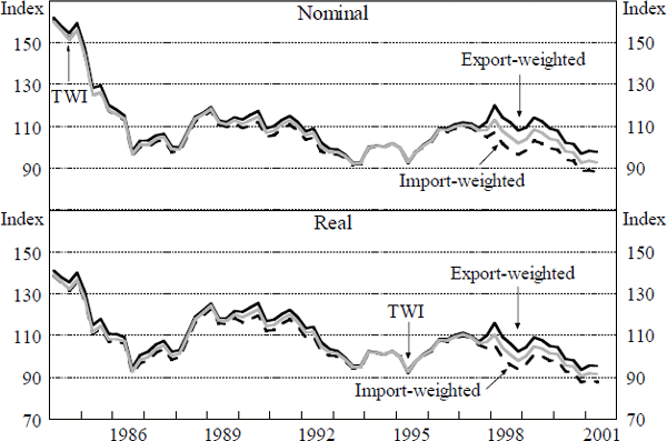
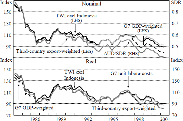
Figures 4 and 5 show a set of quarterly nominal and real exchange rate indices. The data for the trade-weighted, import-weighted, export-weighted and G7 GDP-weighted indices are available at <http://www.rba.gov.au/statistics/>. Data sources are detailed in Appendix A.


It is apparent that different weighting schemes can sometimes result in markedly different results, particularly in the short run. In a few cases, different series do not even agree on the direction of exchange rate movements, let alone the magnitude. This is particularly the case when the home currency is appreciating against some currencies and depreciating against others, as occurred for Australia in 1997 and 1998, and for the major industrialised economies on several occasions.
Similarly, these divergences can affect assessments of the position of the real exchange rate relative to ‘fundamentals’. For example, it has previously been found that the A$ real exchange rate tends to be partly explained over the medium term by fundamental determinants such as the terms of trade (or commodity prices) and real interest differentials (Gruen and Wilkinson 1991; Blundell-Wignall, Fahrer and Heath 1993; Tarditi 1996). We estimate Equation (7) for different measures of the real exchange rate:
where rer is the relevant real exchange rate index, tot is the terms of trade, r is the real cash rate in Australia, and r* is a proxy for the world real interest rate, the weighted average of the real short-term policy rates in the G3 economies.[10] Table 3 shows the results. The differences in the estimated coefficients are not very large in an absolute sense, and the fit of the model is broadly similar regardless of the exchange rate index used. As would be expected, indices with similar weighting schemes – such as the TWI and the TWI excluding Indonesia – give similar results, while the differences between these indices and the export-weighted or GDP-weighted indices are more substantial. By contrast, the price indices used seems less important; the G7 GDP-weighted index deflated by consumer price indices gives very similar results to the index with the same weights deflated by unit labour costs.
| Coefficient | ||||||
|---|---|---|---|---|---|---|
| Exchange rate | β1 | β2 | β3 | β4 | β5 |  |
| Trade-weighted | 0.2874 (0.883) |
−0.3201 (−4.011) |
0.2543 (2.396) |
0.0087 (3.682) |
1.2236 (6.736) |
0.5487 |
| TWI (excl Indonesia) | 0.3526 (1.098) |
−0.2959 (−3.986) |
0.2152 (2.152) |
0.0095 (3.937) |
1.2570 (7.040) |
0.5592 |
| Import-weighted | 0.3850 (1.219) |
−0.3037 (−4.010) |
0.2152 (2.153) |
0.0092 (3.906) |
1.2702 (7.247) |
0.5700 |
| Export-weighted | 0.1808 (0.520) |
−0.2904 (−3.734) |
0.2492 (2.306) |
0.0078 (3.151) |
1.1709 (5.972) |
0.5044 |
| G7 GDP-weighted | 0.5237 (1.613) |
−0.2448 (−3.409) |
0.1245 (1.217) |
0.0095 (3.871) |
1.4176 (7.955) |
0.5687 |
| Unit-labour-cost basis | 0.2709 (0.797) |
−0.2461 (−3.660) |
0.1805 (1.727) |
0.0092 (3.606) |
1.4110 (7.552) |
0.5672 |
|
Notes: Estimation period: 1985:Q1–2000:Q2. Numbers in parentheses are t-statistics. |
||||||
A similar divergence occurs when using different measures of the exchange rate as explanators in other econometric equations. For example, movements in the nominal exchange rate explain much of the variability in import prices (Beechey et al 2000). Table 4 compares the results from an import-price equation with the same structure as that in Beechey et al (2000), using different measures of the exchange rate.[11] The equation takes the form:
| Coefficient | |||||||||
|---|---|---|---|---|---|---|---|---|---|
| Exchange rate measure | ϕ1 | ϕ2 | ϕ3 | ϕ4 |  |
 |
ϕ7 | ϕ8 |  |
|
Notes: Numbers in parentheses are t-statistics. For |
|||||||||
| Trade-weighted | 1.3070 (1.679) |
−0.2766 (−2.191) |
0.1563 (0.647) |
−0.1528 (−1.192) |
0.9120 (*) |
−0.8154 (***) |
−0.0119 (−0.913) |
−0.0004 (−0.595) |
0.7344 |
| TWI (excl Indonesia) | 1.4496 (2.082) |
−0.3820 (−3.195) |
0.3786 (1.709) |
−0.2839 (−2.351) |
0.8048 (*) |
−0.8101 (***) |
−0.0107 (−1.154) |
−0.0011 (−1.816) |
0.7980 |
| Import-weighted | 1.6064 (2.272) |
−0.3977 (−3.280) |
0.3944 (1.784) |
−0.3190 (−2.549) |
0.7912 (*) |
−0.8126 (***) |
−0.0116 (−1.282) |
−0.0010 (−1.869) |
0.7973 |
| Export-weighted | 1.0188 (1.168) |
−0.1508 (−1.186) |
−0.0913 (−0.367) |
0.0138 (0.111) |
1.0887 (**) |
−0.7979 (***) |
−0.0267 (−1.479) |
0.0004 (0.592) |
0.6550 |
| G7 GDP-weighted | 1.6080 (2.809) |
−0.5126 (−4.860) |
0.6950 (3.429) |
−0.4796 (−4.543) |
1.0005 (**) |
−0.7206 (***) |
−0.0332 (−3.670) |
−0.0022 (−4.082) |
0.8564 |
| Third-country export weighted |
1.4109 (1.497) |
−0.1819 (−1.304) |
−0.0177 (−0.056) |
−0.1377 (−0.888) |
0.8271 () |
−0.7207 (***) |
−0.0114 (−1.194) |
−0.0001 (−0.276) |
0.7320 |
where pm is import prices, p*x is a measure of world export prices, and e is the nominal exchange rate. The equation also includes a time trend to proxy for the shift towards lower-priced imports from non-G7 countries, and a dummy since June quarter 1998 to capture the effects of discounting by exporters from countries in financial crisis. Data limitations prevent construction of an export price index covering a wide range of countries. The world export price series used in this equation (p*x) is based on the export price indices of the G7 nations. Therefore, at least some of the divergence in the results presented in Table 4 reflects the mismatch between the nominal exchange rates used and the export price index. This simply underlines the importance of using exchange rate indices that are appropriate to the task at hand, rather than relying on a single index for all purposes.
As would be expected, the equation that fits best is the one containing the exchange rate most closely matching the construction of the export price index, that is, the G7 GDP-weighted exchange rate index. The posited long-run relationship is not significant for the trade-weighted index, the export-weighted index and the third-country export-weighted index; this indicates the unsuitability of these indices to explaining import price movements.[12] The trend and dummy terms become less significant when the exchange rate measure incorporates more information from non-G7 trading partners. The dummy for the Asian crisis becomes completely insignificant when the export-weighted and third-country export-weighted indices are used. This is because these indices incorporate large enough weights on countries affected by financial crisis in 1997–1998 – Thailand, Indonesia, Korea and Brazil – so that the exchange rate measure captures the effects of discounting by crisis-country exporters on the world price level, and therefore the dummy is not needed.
Footnotes
This is the equation presented in Beechey et al (2000). Variants on this equation have been used in de Brouwer and O'Regan (1997) and Lowe and Ellis (1997). [10]
See Anderson et al (1987) for a similar exercise using a model of US merchandise trade. [11]
Although theory would suggest we impose static homogeneity in the effects of exchange rates and foreign prices on Australian import prices, we have not done so for this exercise, so that we can demonstrate the effects of the different exchange rate measures on the estimated long-run relationship. [12]


 and
and  , the table shows
whether at least one of the parameters is significant at the