RDP 2005-02: The Impact of Monetary Policy on the Exchange Rate: A Study Using Intraday Data 3. Results
April 2005
- Download the Paper 158KB
3.1 The Impact of Monetary Policy Shocks
To quantify the impact of monetary policy on the exchange rate we regress the change in the exchange rate over the event window on the monetary policy surprise, as represented by Equation (1),
where Δe[t−10m,t+60m] is the
percentage change in the US dollar bilateral exchange rate from 10 minutes
before the event to 60 minutes after, and  is the surprise move
in policy measured by the daily change in market interest rates. We use the
exchange rate from 10 minutes before the policy change, rather than at the
time of the policy change, in case there are mismatches in the timing of our
exchange rate data and policy implementation. We present results using surprises
derived from both 1-month and 3-month interest rates.
These regressions suggest that a 100 basis point surprise tightening of monetary policy is estimated to lead to an appreciation of the exchange rate in the range of 1–2 per cent in the hour following the event (Table 3). When we use the sample pooled across countries the estimate is in the middle of this range, just under 1½ per cent.[5] As noted in Section 2.3, the countries used in this study now move their policy rates in 25 basis point increments. A 25 basis point surprise would lead to an appreciation of ¼−½ per cent. The surprise in monetary policy explains only about 10–20 per cent of the movement in the exchange rate over the 70-minute interval. The low proportion of exchange rate movements explained by the interest rate surprise, even in such a short window, is in line with other work on the exchange rate, for example Andersen et al (2003) and Faust, Rogers, Wang and Wright (2003).
| Country | 1-month | 3-month |  |
Observations |
|---|---|---|---|---|
| Australia | 0.96 (0.00) |
0.16 |
79 |
|
| 1.88 (0.00) |
0.32 |
79 |
||
| Canada | 1.56 (0.00) |
0.22 |
33 |
|
| 1.67 (0.00) |
0.23 |
33 |
||
| NZ | 1.83 (0.02) |
0.11 |
42 |
|
| 1.97 (0.01) |
0.15 |
42 |
||
| UK | 1.04 (0.00) |
0.11 |
82 |
|
| 1.58 (0.00) |
0.17 |
82 |
||
| Pooled sample | 1.45 (0.00) |
0.13 |
222 |
|
| 1.77 (0.00) |
0.17 |
222 |
||
| Notes: The dependent variable is the change in the exchange rate (relative to the US dollar) from 10 minutes before the event to 60 minutes after. P-values are in parentheses. | ||||
For all countries and the pooled sample, the coefficient on the interest rate surprise is larger when the surprise is measured using a 3-month interest rate than in the equivalent regression using a 1-month interest rate. Presumably this is because the 3-month rate includes the impact of the decision on expectations of future monetary policy, at least over the next 3 months, an important issue that we explore in Section 3.2. The point estimates for the 3-month surprises for Australia and Canada are similar to Zettelmeyer's (2004) results using daily data. However, his result for New Zealand is larger, 2.7 per cent, possibly because his sample, being mostly before 1999 when a monetary conditions index was being used, does not contain purely exogenous monetary shocks. The point estimates are also similar in magnitude to the 1.2 for the deutschemark/euro exchange rate response to changes in US interest rates contained in Faust, Rogers, Wang and Wright (2003). However, their estimate for the pound's response to US interest rates of 0.66 is smaller, suggesting that their result may contain some bias in estimating the impact of a change in a large country's interest rate on the bilateral exchange rate with a smaller country.
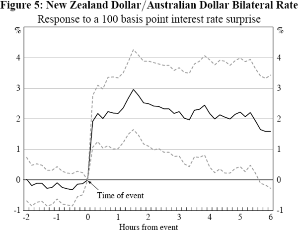
The timing of the impact of a monetary policy surprise on the exchange rate can be determined by estimating Equation (2) for k ranging from 2 hours before the event to 6 hours after (at 10 minute intervals).
The results are shown in Figures 1 to 4 where the surprise is measured using the 1-month interest rate. In all 4 countries there is a sharp spike in the impact in the 10 minutes following the event, demonstrating that monetary policy announcements have a rapid impact on the exchange rate. The relative stability of the coefficients over the six hours after the event indicate that the surprise has little additional influence after its immediate impact. The standard errors, the dashed lines in the graphs, widen further from the event as the policy change becomes a smaller proportion of the information incorporated into the exchange rate. As a result, the statical significance using daily data will be substantially weaker.
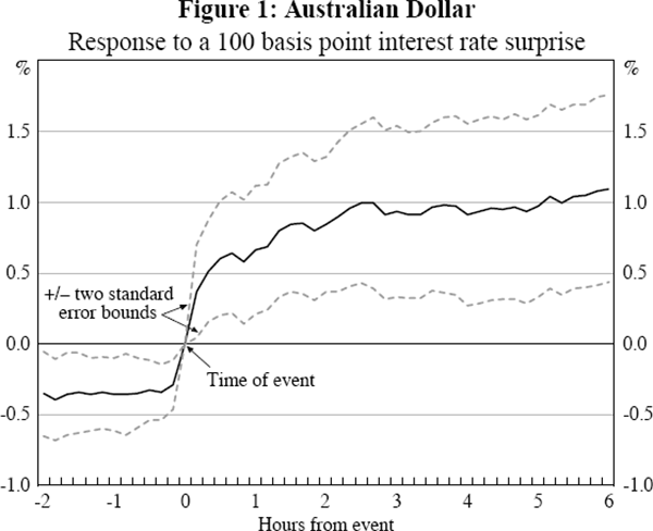
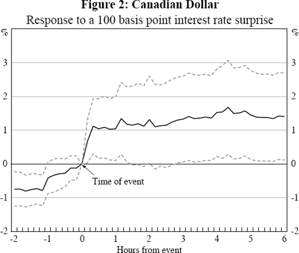
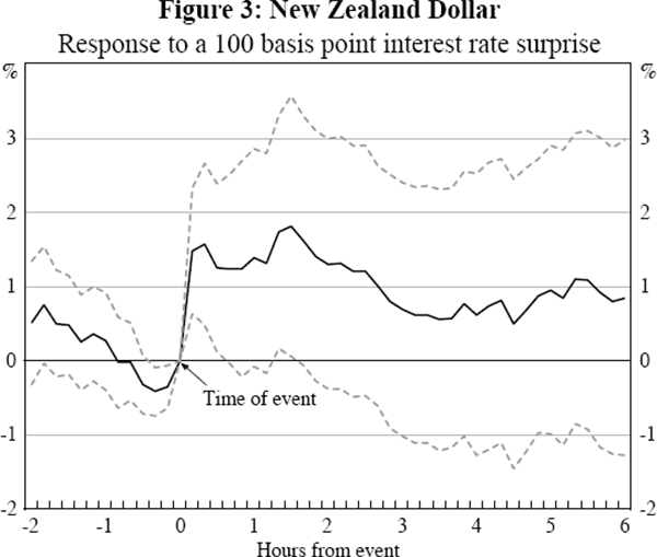
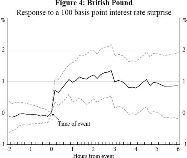
For Australia and Canada there is significant movement in the exchange rate prior to the event in the same direction as the response following the event. Given this is gradual for Canada it is suggestive of late changes in market expectations of the policy announcement, perhaps as participants' expectations coalesce around a particular policy announcement. Such changes in market expectations would presumably also be reflected in intraday interest rate data were they available. For Australia the sharp jump that occurs 10 minutes before the event most likely reflects slight differences between the timing of the announcement and the exchange rate data. The significance of this change immediately prior to the event is not unduly influenced by any particular observations and so the result does not appear to be the result of leaked information.[6] It is because of this possible timing mismeasurement that we base our main results on the exchange rate starting 10 minutes before the event.
Given the importance for New Zealand of financial linkages with Australia, and New Zealand's smaller relative size, it is also interesting to examine the impact of monetary policy surprises in New Zealand on the New Zealand dollar/Australian dollar bilateral exchange rate. Figure 5 demonstrates that the response is more precisely estimated, and larger, than for the response of the New Zealand dollar/US dollar exchange rate shown in Figure 3.
3.2 The Importance of Expectations
The impact of a policy decision on expectations of future policy may be important in determining the exchange rate's response. This is apparent from the different results obtained when measuring the monetary policy surprise using 1-month and 3-month interest rates. A monetary policy decision might simply surprise the market in its timing (a ‘timing’ surprise), or it might be a surprise that shifts policy expectations at all horizons (a ‘level’ surprise). A change in current monetary policy could even shift expectations of future policy by more than the impact on 1-month interest rates if market participants believe that it indicates that future changes in the same direction are likely.
To test whether expectations are important we examine changes in 3-month interest rate futures (details of these contracts are in Appendix A). These are not perfect measures of policy expectations, but changes in these interest rates have been shown to be a reasonable guide to changes in policy expectations (Piazzesi and Swanson 2004). Typically, about eight futures contracts trade at any one time, giving a horizon of about two years in total. What is termed the ‘first’ interest rate futures contract expires sometime in the next 3 months, and is settled on the 3-month interest rate prevailing on that expiration date. The ‘second’ futures contract is settled on the 3-month interest rate prevailing 3 months after the expiration of the first contract, and so on. Because the futures contracts expire at fixed points in time 3 months apart, but monetary policy events can happen at any time in a 3-month period, the horizon until the contract expiration can differ from 1 event to another. While not ideal, this is unavoidable given that 1-month futures contracts are not available for these countries over the relevant sample and the time between the fixed announcement dates can vary in Canada and New Zealand. We consider the sensitivity to this measurement issue in Section 3.3.
Figure 6 shows a scatterplot of the change in the 1-month interest rate against the change in the second futures contract, on days with a monetary policy event, for all four countries. We use the second futures contract as it has the advantage that it does not expire until after at least two complete monetary policy decision cycles.
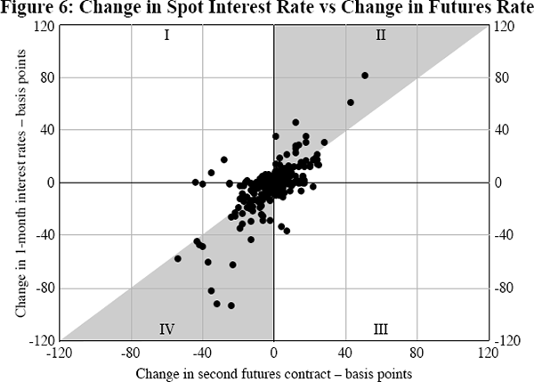
Given that monetary policy changes are not quickly reversed, surprises that lead to a positive (negative) change in the 1-month interest rate are unlikely to also lead to a negative (positive) change in the futures rate. This suggests that there should be very few points in Quadrants I and III. It would seem likely that most surprises would be somewhere between a level and timing surprise. Changes in the futures rate should then be of the same sign as, but smaller in magnitude than, the change in the 1-month rate. In this case, most observations would lie in the shaded area in Figure 6. The data broadly fit this pattern, especially for large monetary surprises, although there are still quite a number of points outside the shaded area. If all surprises had the same effect on expectations of future policy then they would lie on a straight line. The scatterplot shows that this is clearly not the case, and regressions for each country indicate that the change in the 1-month interest rate explains only about half of the change in the second futures rate. It thus appears that there is sufficient heterogeneity to test whether the effect that a monetary policy decision has on expectations of future policy is important in determining the decision's impact on the exchange rate.
We incorporate information on the change in the futures contract in Equation (3).
A ‘timing’ surprise – a surprise that does not change expectations
of the level of future policy – is captured by β, since there is no change in the futures interest rate (that
is,  ).
A ‘level’ surprise – a surprise that changes expectations
of future interest rates by as much as the surprise in current policy, i.e.,
 – is measured by β + γ. The results are presented
in Table 4.
|
Timing surprise β |
γ |
Level surprise β + γ(a) |

|
Observations | |
|---|---|---|---|---|---|
| Australia | 0.46 (0.14) |
0.80 (0.02) |
1.26 (0.00) |
0.21 |
79 |
| Canada | 0.84 (0.26) |
0.85 (0.20) |
1.69 (0.00) |
0.23 |
33 |
| NZ | 1.06 (0.35) |
0.74 (0.35) |
1.80 (0.02) |
0.11 |
42 |
| UK | −0.21 (0.59) |
2.44 (0.00) |
2.22 (0.00) |
0.29 |
82 |
| Pooled sample | 0.87 (0.00) |
0.81 (0.00) |
1.68 (0.00) |
0.17 |
222 |
| Notes: P-values are in parentheses. (a) The p-value for β + γ is calculated using a Wald test. |
|||||
These results confirm that a surprise in the level of policy leads to a greater change in the exchange rate than does a surprise in the timing of policy. Estimates of the impact of a 100 basis point surprise in timing, β, for the individual countries are imprecisely estimated, but range from being negative to around 1 per cent. However, in the larger pooled sample, the estimate is very precisely estimated to be 0.87. A 100 basis point surprise increase in the level of the (current and future) policy instrument is estimated to lead to a 1.3 to 2.2 per cent appreciation in the exchange rate, as seen by the estimates of β + γ. The pooled sample produces an estimate in the middle of this range, 1.68. These estimates of the impact of a level surprise are highly significant for all of the countries and the pooled sample. This indicates that a 25 basis point timing (level) surprise would appreciate the exchange rate by around 0.2 per cent (0.4 per cent). Clearly a level surprise has a much larger impact on the exchange rate than a timing surprise.
It is interesting to benchmark these results to what the theory of UIP might suggest. To calculate the jump in the exchange rate that would be implied by a surprise change in monetary policy, we need to know both how long the change in monetary policy will be sustained and the level that the exchange rate is expected to return to after the change in the interest differential is undone. Using our estimates that separate the timing from the level effects we can attempt to control for the first of these issues. But without knowing what caused the monetary surprise, and what impact that news had on the equilibrium value of the exchange rate, we cannot determine the level to which the exchange rate is expected to return. For the purpose of this calculation we assume that the monetary surprise did not change the long-run expected value of the exchange rate. If the monetary decision is a pure timing surprise, the interest rate given by the futures contract that expires in 3–6 months does not change. Assuming that the surprise lasts 4½ months (that is, the midpoint of 3 and 6 months), UIP suggests that a 100 basis point surprise increase would lead to an immediate appreciation of less than half a per cent (0.375 per cent).[7] In contrast we estimate the response to a 100 basis point timing surprise to be over twice as large, 0.87 per cent. Of course, this interpretation is subject to the important caveat that we do not know how the long-run equilibrium level of the exchange rate has changed.
3.3 Robustness
To test the robustness of our findings we include a range of other variables in the regressions. For brevity we only report results using the pooled sample. The equivalent regressions for the individual countries produce similar results, though understandably with larger standard errors. Table 5 reports specifications using surprises based on 1-month bank bill interest rates, while Table 6 repeats the regressions using surprises based on 3-month bank bill rates. The coefficients on monetary policy surprises are found to be robust and maintain their statistical significance across a range of specifications. Specifications I and II repeat the pooled results from Tables 3 and 4. The estimates using the 3-month interest rate surprise are slightly larger, reflecting their less precise separation of timing and level surprises. Using the third rather than second futures contract, Specification III, does not change the results appreciably.
| Model |
Surprise change β |
Futures contract γ |
Expected change | Maturity(a) | Change dummy with: |  |
||
|---|---|---|---|---|---|---|---|---|
| 2nd | 3rd | Surprise change | 2nd future | |||||
| I | 1.45 (0.00) |
0.13 |
||||||
| II | 0.87 (0.00) |
0.81 (0.00) |
0.17 |
|||||
| III | 0.95 (0.00) |
0.74 (0.00) |
0.17 |
|||||
| IV | 0.89 (0.00) |
0.83 (0.00) |
−0.21 (0.00) |
0.18 |
||||
| V | 0.94 (0.00) |
0.76 (0.01) |
−0.21 (0.09) |
0.00 (0.61) |
0.17 |
|||
| VI | 0.61 (0.16) |
0.72 (0.01) |
−0.25 (0.06) |
0.00 (0.61) |
0.58 (0.26) |
0.17 |
||
| VII | 0.74 (0.10) |
0.47 (0.19) |
−0.24 (0.06) |
−0.01 (0.46) |
0.15 (0.82) |
0.63 (0.26) |
0.18 |
|
| Notes: The dependent variable is the change in the exchange rate (relative
to the US dollar) from 10 minutes before the event to 60 minutes after.
P-values are in parentheses. There are 222 observations in all regressions. (a) The maturity variable is: (the change in the futures contract) × (the difference between the days to maturity and the average days to maturity). |
||||||||
| Model |
Surprise change β |
Futures contract γ |
Expected change | Maturity(a) | Change dummy with: |  |
||
|---|---|---|---|---|---|---|---|---|
| 2nd | 3rd | Surprise change | 2nd future | |||||
| I | 1.77 (0.00) |
0.17 |
||||||
| II | 1.27 (0.00) |
0.52 (0.08) |
0.18 |
|||||
| III | 1.32 (0.00) |
0.48 (0.07) |
0.18 |
|||||
| IV | 1.32 (0.00) |
0.51 (0.08) |
−0.21 (0.08) |
0.19 |
||||
| V | 1.42 (0.00) |
0.41 (0.22) |
−0.20 (0.10) |
−0.01 (0.49) |
0.18 |
|||
| VI | 0.94 (0.08) |
0.39 (0.24) |
−0.23 (0.06) |
−0.01 (0.48) |
0.72 (0.20) |
0.19 |
||
| VII | 1.01 (0.08) |
0.30 (0.45) |
−0.23 (0.06) |
−0.01 (0.45) |
0.49 (0.54) |
0.25 (0.71) |
0.18 |
|
| Notes: The dependent variable is the change in the exchange rate (relative
to the US dollar) from 10 minutes before the event to 60 minutes after.
P-values are in parentheses. There are 222 observations in all regressions. (a) The maturity variable is: (the change in the futures contract) × (the difference between the days to maturity and the average days to maturity). |
||||||||
One surprising result is that the coefficient on the expected change (the change in monetary policy less the unexpected change) is always about −0.2 per cent and marginally significant (Specifications IV–VII). This runs counter to our priors that only unexpected changes in monetary policy should affect the exchange rate. This result owes a lot to one particular event in New Zealand, 17 May 2000. The tightening in monetary policy on this day was almost completely anticipated. But the particularly hawkish Monetary Policy Statement released with the decision seemingly led to concerns about the impact of the indicated course of policy on the growth of the economy and a sharp depreciation of the exchange rate. Excluding this observation, the expected change in policy does not have a statistically significant impact on the exchange rate.
A variable that controls for the changing number of days until maturity of futures contracts, used in Specifications V–VII, is always economically and statistically insignificant. This suggests that our conclusions about the timing and level surprises are not unduly influenced by the fact the horizon of interest rate futures is not constant across events.
The coefficient on a dummy for whether the decision was a change in monetary policy, multiplied by the monetary policy surprise, is always positive though not significant (Specifications VI and VII). This suggests that there may be a slightly greater effect on the exchange rate when the surprise monetary decision is a change in the policy interest rate. Alternatively, this could simply reflect the fact that the proportion of the interest rate change that is caused by monetary policy is likely to be higher when the surprise is larger, which typically occurs when monetary policy is changing.
Footnotes
The data do not reject the restriction that the coefficient on interest rates is constant across countries. [5]
This result is not sensitive to the exclusion of the only two events for Australia in which there is any suggestion of some participants seemingly having early access to the policy outcome: one in which the monetary policy decision was mistakenly released to some market participants six minutes early (2 February 2000) and the other in which Bloomberg mistakenly released a report about one minute early even though it did not yet know the outcome (3 July 2002). Note that these do not affect our main results because we use the exchange rate from 10 minutes before the policy change. [6]
This assumes that the foreign interest rate remains constant. [7]


