RDP 2005-04: Monetary Policy, Asset-Price Bubbles and the Zero Lower Bound Appendix B: The Phase Diagram for the Ball-Svensson Model Under Optimal Policy

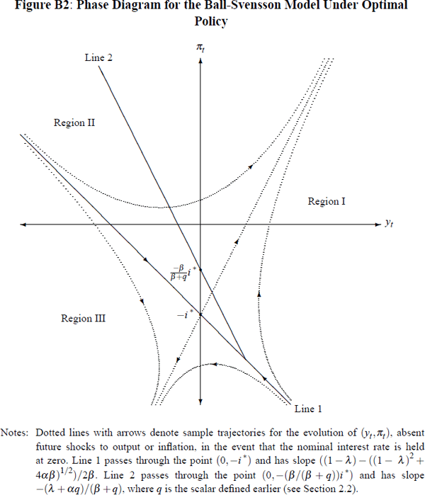
In this appendix we outline the derivation of the phase diagram (Figure 1) discussed in Section 3 of the main body of the paper. This phase diagram is replicated in Figure B2, now for the case of general model and loss function parameters α, β, λ and μ. Note that this phase diagram represents a particular case of that derived previously, by Reifschneider and Williams (2000), for the Ball-Svensson model with policy determined by a general Taylor Rule.^[24]

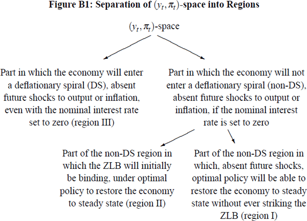
The basic idea of this phase diagram is that we can separate (y_t,π_t)-space into three distinct components, as shown in Figure B1:

We begin by establishing the existence and properties of region III. To this end observe that, in the absence of future shocks to output or inflation, the evolution of our Ball-Svensson economy may be described, in terms of nominal interest rates, by the system

where the matrix M, and the vectors Z_t and X_t, are defined by

Now consider the question: what initial conditions for Z would result in the economy entering a deflationary spiral, even in the event that i^lvl were held at the ZLB? To answer this question note that, for i^lvl = 0, Equation (B1) may be rewritten more simply as:

where W_t denotes the vector W_t = (y_t,π_t + i*)^T. Then, for this simplified system, the evolution of any initial W_t is clearly determined simply by the eigenvalues, ξ_±, and eigenvectors, ν_±, of the matrix M, which are readily computed to be:

and

Note that, for α,β,λ > 0, then ξ₊ will clearly satisfy ξ₊ > 1; while ξ₋ will satisfy 0 < ξ₋ < 1 provided λ αβ (which holds for our baseline choice of model parameters: α = 0.4, β = 1.0 and λ = 0.8).

Hence, translating back to (y_t, π_t)-coordinates, we see that (y_t, π_t)-space may be split into two halves, in one of which the economy will enter a deflationary spiral even with nominal interest rates set to zero, as shown in Figure B2. The line separating these two halves passes through the point (0, −i*), and has slope equal to that of the eigenvector ν₋, namely ((1−λ) − ((1−λ)² + 4αβ)^½)/2β. This slope is approximately −0.54 for our baseline choice of model parameters.

In addition, the non-deflationary-spiral component of (y_t, π_t)-space may itself be sub-divided into two parts: one where the ZLB will initially be binding on optimal policy (region II); and one (region I) where it will not be binding (so that, absent future shocks, the economy may be returned to steady-state without ever setting nominal interest rates to zero).

The dividing line between these two regions will simply be given by the set of states (y_t, π_t) for which the associated unconstrained optimal nominal interest rate recommendation exactly equals zero. Yet we know that, for any given levels of the output gap and inflation, the unconstrained optimal real interest rate recommendation is simply:

where the scalar q is defined by q = (− μα + (μ²α² + 4μ)^½)/2. Hence, since = + π_t + π*, the dividing line between regions I and II will be precisely the line

or, in other words,

Note that this passes through the point (0,−(β/β + q)i*) and has slope −(λ + αq)/(β + q), as shown in Figure B2.

This completes the derivation, for general model and loss function parameters, of the phase diagram for the Ball-Svensson model under optimal policy.^[25]

Footnotes

Here we consider only the case where policy is set optimally, which turns out to be a specific instance of a Taylor Rule – see Equation (12). [24]

While we do not pursue this further here, it is also possible to use this phase diagram (Figure B2) to better understand the precise way in which being in region II will result in additional loss for a policy-maker, over and above that which they would expect to incur in the absence of the ZLB. The key observation is that, without the ZLB, our Ball-Svensson economy will evolve under optimal policy according to the equation Z_t =UZ_t−1 where U is a 2×2 matrix with eigenvalues 0 and (1 − αq). Computation of the corresponding eigenvectors, which turn out to be (1,α)^T and (q,−1)^T respectively, allows the way in which optimal policy moves the economy around in (y_t, π_t)-space to be easily pictured – and hence, in turn, allows the impact of the ZLB on a policy-maker, trying to stabilise an economy in region II, to be understood geometrically in terms of the phase diagram. [25]