RDP 2006-10: The Performance of Trimmed Mean Measures of Underlying Inflation 5. Empirical Analysis
December 2006
- Download the Paper 329KB
A number of criteria have been proposed as desirable for measures of underlying inflation. Some of these relate to the production and dissemination of measures, for example that they should be timely and verifiable (Roger 1997), understandable by the general public, computable in real time, and not subject to revision (Wynne 1999). We take it as given that both trimmed mean measures and exclusion measures satisfy these criteria. Other criteria are more empirical: for example, Roger suggests that measures should be ‘robust and unbiased’ while Wynne suggests they should be ‘forward looking in some sense’. In this section we focus on some empirical criteria, as discussed in Section 2. For the most part, these can be viewed as various ways of searching for underlying measures that meet Blinder's (1997) goal of better identifying the signal from the noise.[21]
5.1 Smoothness of Underlying Inflation Measures
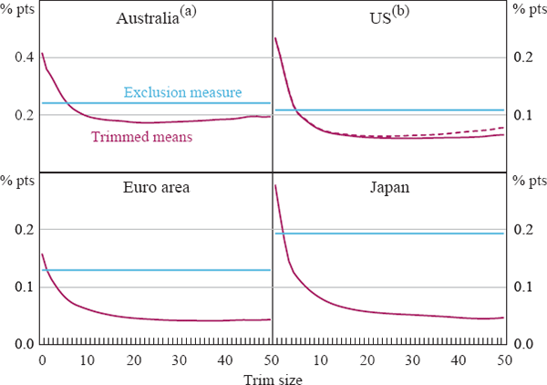
One way to assess smoothness is to examine which measures are more persistent. An alternative is to examine the smoothness of different measures, based on the standard deviations of period-to-period changes in monthly or quarterly inflation rates. Figure 4 presents these data for the headline CPI (represented by the 0 per cent trim), the exclusion measure (shown as a horizontal line), and for the various trimmed means for trims from 1 to 50 per cent. The results are fairly consistent across economies. They suggest that as we increasingly trim price changes from either end of the distribution we obtain a much smoother measure of high-frequency inflation. Most of the gains in smoothness have been obtained after about 10 per cent of the distribution has been trimmed from either end. The lowest point for each line corresponds to the smoothest measure, which represents a reduction in volatility of around 60–85 per cent, with larger reductions for the economies with monthly data. The trims that would appear ‘optimal’ (on this criterion) differ but are all in the range of about 20–40 per cent. However, for all economies there is a fairly wide range of trims that offer broadly similar improvements in smoothness. The exclusion measures are also smoother than the headline CPI measures, as shown by the level of the horizontal lines. However, in all cases they offer much less reduction in noise than most of the trimmed mean measures.
Notes:
(a) Quarterly inflation.
(b) Dashed line is calculated without disaggregating the implicit rent component.
The results for the US also provide some initial evidence on the performance of trimmed mean measures when the implicit rent component is broken into four sub-components (shown by the solid trimmed means line in the top right-hand panel of Figure 4). The difference is relatively small for small trims, but it increases for larger trims. For the weighted median (or 50 per cent trim), disaggregating the implicit rent component results in a measure that is about 15 per cent smoother than when it is not broken up.
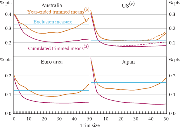
We can also use the smoothness criterion to shed light on the relative merits of trimmed mean measures calculated from short-horizon and longer-horizon changes. In Figure 5 we show information on the smoothness of annual measures of inflation, calculated from the distribution of annual price changes and from the cumulated monthly or quarterly trimmed means used through most of this paper. The results suggest that cumulated monthly or quarterly changes provide much smoother measures of annual inflation than measures based on the distribution of annual changes. The gains from using cumulated measures are much larger for larger trims, and in some cases the weighted medians based on annual changes do not perform well at all.[22] Accordingly, these results argue against the use of weighted medians based on the year-ended distribution of price changes.
Notes:
(a) Constructed from distributions of monthly/quarterly inflation.
(b) Constructed from distributions of year-ended inflation.
(c) Dashed lines are calculated without disaggregating the implicit rent component.
5.2 Bias with Respect to Headline Inflation
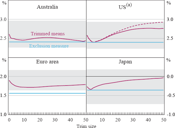
Figure 6 shows average annualised rates of underlying inflation for the four economies. To provide some perspective on the observed differences in inflation rates, we also include a simple estimate of the 95 per cent confidence interval around the mean growth for the headline CPI.[23] The results for all four economies indicate that the trimmed mean measures typically have a fairly similar mean inflation rate to the headline CPI (again, this is the 0 per cent trim measure). The largest difference is for the standard weighted median for the United States which has a mean annualised growth rate which is 0.34 percentage points higher than the rate for the headline CPI. However, when we disaggregate the implicit rent component the difference falls to only 0.18 percentage points. In general, the absolute differences in mean growth rates relative to the CPI tend to be lower for central trims such as the 25 per cent trimmed mean than for the weighted median. In addition, the average growth rates for the trimmed means are sometimes above (the United States and Japan) and sometimes below (Australia and the euro area) the average growth of the headline CPI, whereas the average growth rate of the exclusion measure is in all cases below the growth of the headline CPI. The latter is not surprising given the increase in real energy prices over the sample period.
Notes:
Shaded areas indicate 95 per cent confidence interval around mean CPI (0 per cent trim)
inflation.
(a) Dashed line is calculated without disaggregating the implicit rent component.
There would seem to be a number of ways that one could do formal statistical tests for bias with respect to the headline CPI.[24] Such tests provide mixed evidence regarding the hypothesis of unbiasedness for the trimmed mean measures (and for the exclusion measures). However, formal statistical tests for unbiasedness must be somewhat tentative over relatively short periods of 10–15 years, especially at times of large movements in fuel prices at the end of the sample period. In cases such as these, reasonable people might differ as to how to interpret a difference in average growth rates between an underlying measure and the headline CPI: perhaps additional data will suggest that any differences in growth rates reflected anomalous movements in the headline CPI. Accordingly, given that the differences in average rates of growth appear relatively small (positive for two economies but negative for the other two), we would characterise the trimmed means for these economies as appearing to be unbiased measures.[25]
5.3 Closeness to Trend Inflation
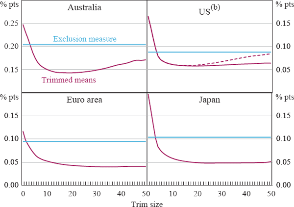
In this section, we calculate the root mean squared error (RMSE) of the candidate measures versus a measure of trend inflation. The trend is defined as the centred 25-month moving average of CPI inflation for the United States, Japan and the euro area, and the 9-quarter moving average for Australia. The results are shown in Figure 7 and are reasonably consistent with the earlier analysis of smoothness. In all four cases, even small trims result in a substantial reduction in the RMSE relative to trend inflation. The maximum reductions in RMSE range from 65–75 per cent for the economies with monthly data and about 40 per cent for Australia's quarterly data. For each economy there is a wide range of trims offering substantial improvements relative to both the headline CPI and the exclusion-based measure. The ‘optimal’ trims (according to this measure) are around 15–35 per cent. Again, the US trimmed means calculated using disaggregated data for implicit rent outperform the aggregated measure, especially as we move towards the weighted median.
Notes:
(a) 25-month- or 9-quarter-centred moving average of CPI inflation.
(b) Dashed line is calculated without disaggregating the implicit rent component.
5.4 Ability to Predict Near-term Inflation
A number of researchers (for example, Cogley 2002) have assessed measures of underlying inflation by how well they forecast inflation over periods as long as three years (or even five years in the case of Bryan and Cecchetti 1994). The rationale is often that this is the horizon of ‘greatest relevance to monetary policy’. However, we do not consider predictability over such long horizons to be a sensible test.[26] Consider the case where a central bank had a good measure of underlying inflation to help inform its policy process. Hence when the measure indicated a build-up in underlying inflationary pressures the central bank would tend to respond by tightening monetary policy, placing downward pressure on inflation over the next two to three years. So we would not expect to see any predictability from underlying inflation to headline inflation at relatively long horizons. More generally, over periods of two or three years, developments in inflation will be determined by movements in the fundamental economic determinants of inflation, including the influence of monetary policy.
Instead, as discussed in Section 2, we think it is more plausible that any predictability is likely to be a fairly short-term phenomenon. Accordingly, we instead examine whether CPI inflation over three or six months (or one or two quarters) can be predicted by various measures of underlying inflation over the corresponding preceding period. The first exercise we conduct is to assess the performance of a rule that simply uses various measures of lagged inflation as the prediction for future headline inflation, so that we can calculate the RMSE for each underlying measure i as given by:
where  denotes inflation in measure i over the k
periods to time t.
Some researchers, starting with Bryan and Cecchetti (1994), have conducted similar tests using a regression framework, that is, allowing for the possibility of a coefficient on the lagged underlying inflation rate that is different to one (and a non-zero constant term). However, other researchers (for example, Rich and Steindel 2005) have found that the results of such exercises can differ significantly between in- and out-of-sample tests, with some instability in coefficient estimates. In contrast, our estimates may be more robust in the sense that there is no difference between in- and out-of-sample tests. Equivalently, our analysis corresponds to feasible forecasting rules that might be quite close to those followed by real-world analysts, who might well forecast that near-term CPI outcomes will be similar to recent underlying inflation outcomes.[27]
Of course, if headline inflation is very noisy it raises the question of whether the ability to forecast it is a particularly useful test of underlying measures. Instead, if there exist other measures that seems to better reflect the trend in inflation, perhaps it might be a better test to see which of the candidate measures of underlying inflation can best predict these other measures. Accordingly, we also assess how well our various measures of underlying inflation can predict either the exclusion measure of underlying inflation or the 25 per cent trimmed mean.
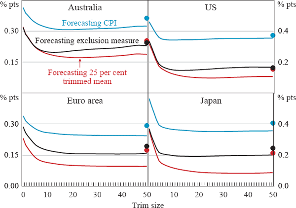
The results for the three-month (or one-quarter) horizon are shown in Figure 8 and indicate that the use of trimmed means for forecasting headline inflation result in reductions in RMSE of 25–40 per cent relative to forecasting with headline inflation itself. As was also the case for the other criteria, most of the gains accrue after only a relatively small amount of trimming. ‘Optimal’ trims according to this criterion vary from around 10 per cent for the United States to nearly 50 per cent for the euro area. As with other criteria, for each economy there is a wide range of trimmed means that perform substantially better than either the headline or exclusion measures.[28]
Notes: Dots show forecast performance of exclusion measures
The results show a substantially lower RMSE for forecasting the two measures of underlying inflation, indicating that these measures of underlying inflation are more forecastable than the headline CPI. Interestingly, the trimmed mean measures tend to outperform the exclusion measure in forecasting the exclusion measure. The smallest forecast error occurs when the trimmed mean measures are used to forecast the 25 per cent trimmed mean inflation rate. The RMSEs from this exercise are up to 60–85 per cent lower than the RMSEs when the CPI is used to forecast itself.
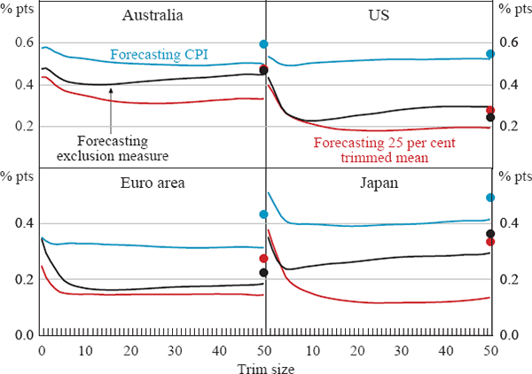
The results for the six-month (or two-quarter) horizon are shown in Figure 9 and indicate smaller gains from using trimmed means to forecast the CPI. Nevertheless, the use of trims results in reductions of up to about 10–25 per cent in RMSE terms. However, the overall modest improvements in RMSEs suggest that central banks wanting to improve forecasts for the CPI at horizons of six months or more are likely to rely more on economic models and other information than simply on the current level of underlying inflation.
Notes: Dots show forecast performance of exclusion measures
The second assessment of predictability uses Granger causality tests between headline CPI inflation, exclusion measures, and 25 per cent trimmed mean inflation. For Australia, we test for Granger causality in quarterly inflation. For the other three economies, we look through the noise in monthly data by using inflation over three-month periods (period t to t+3) and we use non-overlapping lagged three-month inflation (t-3 to t) as the explanatory variable.[29] The results are shown in Table 1.[30]
| Direction of Granger causality test | Australia | Euro area | Japan | US |
|---|---|---|---|---|
| Headline to trimmed mean | No | No | No | No |
| Headline to exclusion | No | No | No | No |
| Trimmed mean to headline | Yes | Yes | No | No |
| Trimmed mean to exclusion | Yes | Yes | No | Yes |
| Exclusion to headline | No | No | No | No |
| Exclusion to trimmed mean | No | No | No | No |
The tests show that there is usually no evidence for Granger causality, with the exception that trimmed mean inflation Granger causes headline inflation for two of the four economies and Granger causes the exclusion measure in three of the four economies. Our interpretation of the results, based on the framework discussed in Section 2, is as follows. In an ideal world, since these variables can all be viewed as proxies for true unobservable underlying inflation, we might expect to see bi-directional Granger causality in most cases. However, in short samples and with significant amounts of noise, especially in the headline CPI, it would not be surprising if we frequently fail to find Granger causality. Cases where we do find Granger causality are likely to be where a relatively good estimate of underlying inflation has information that helps predict a more noisy (but not excessively noisy) measure. This is consistent with the results that show that trimmed mean inflation often Granger causes other measures of inflation, but that there is no Granger causality from either of those other two measures.
It is noteworthy that the goodness of fit in the equations for forecasting the CPI is typically quite low. One interpretation might be that underlying measures – both trimmed mean and exclusion measures – are of limited value because their ability to forecast headline inflation is only modest. An alternative interpretation would be that it is exactly because of the noise in headline inflation – most visible in Figure 3 – that we need measures of underlying inflation, and that their primary function is as guides to the current level of inflationary pressures rather than as leading indicators of future headline inflation. We tend to favour the latter view, and suggest that the predictability results and earlier exercises in this section present a powerful case for the trimmed mean measures being much closer to an optimal measure of underlying inflation than either the CPI or the exclusion measures.
Footnotes
It is easily shown, based on the framework in Equation (1) and plausible assumptions about some variances and covariances, that the criteria in Sections 5.1, 5.3 and 5.4 are all driven by the variance of the idiosyncratic term in Equation (1). [21]
The reason for the relative volatility of the weighted median is that even at the centre of the ordered distribution, there can sometimes be noticeable gaps in the annual inflation rates of adjacent items, so the annual weighted median can be quite volatile. This may contribute to the finding by Armour (2006) that Canadian weighted median inflation (calculated using the year-ended distribution) is more volatile than some other underlying measures. It is noteworthy that the Reserve Bank of New Zealand's trimmed mean measure, which is based on the distribution of annual price changes, trims only 5 per cent of the distribution at either end. [22]
The confidence interval is the standard one under the assumption that monthly/quarterly inflation rates are drawn from a normal distribution, namely μ ± (t-stat*σ)/√N, where the standard deviation is calculated using high-frequency inflation rates then annualised. We use this mostly to give readers some common simple metric of whether deviations in growth rates are relatively large or small. [23]
There is relatively little discussion in earlier research as to how to test for bias. At least three possibilities suggest themselves. First, one could calculate simple confidence intervals as in Footnote 23 and shown in Figure 6. Second, there is the standard approach of regressing underlying inflation on a constant and the headline rate (or vice versa) and testing the hypothesis that the constant is zero and the slope coefficient is unity. Third, one could test for cointegration and a unit elasticity between the levels of underlying and headline price indices. The first may not be entirely appropriate as the time series properties of the noise in headline inflation may render the assumption of normality invalid. The second seems inappropriate because it is less a test of similarity of long-run growth rates and more a test of period-by-period correlations. The third seems most appropriate in principle, but may suffer from the usual problems of running cointegration tests over relatively short samples. [24]
However, in analysis not presented in this paper we have also calculated trimmed mean measures for the UK and found evidence of substantial bias as we move towards the weighted median. As Catte and Sløk (2005) have noted, this may be because services prices tend to be less volatile than goods prices and are trimmed less frequently, and because the gap between goods and services inflation has been somewhat larger in the UK than elsewhere. Of course, a biased measure can still provide useful information; if the bias is relatively constant, the measure may still be a useful indicator of changes in underlying inflation. Indeed, trimmed mean measures for the UK appear to generally perform reasonably well in other tests. [25]
Some of our reservations appear to be also shared by Wynne (1999). [26]
Others who have used our approach include Cutler (2001) and Vega and Wynne (2003). [27]
Of course, the similarity of these results with those in Section 5.2 is not surprising. As Vega and Wynne (2003) have noted, a measure that does well in tracking a centred moving-average trend should also do well in explaining a forward-looking trend. [28]
For the monthly data, the tests use overlapping data to improve the efficiency of the parameter estimates: we use Newey-West errors to control for the moving average error term that is introduced. The equations all contain just one lag, the maximum that is suggested by the data. [29]
All results are valid at the 5 and 10 per cent levels. There is one judgmental adjustment in the case of the test for whether Japanese headline inflation Granger causes trimmed mean inflation. When we add lagged headline inflation to an equation with just lagged trimmed mean inflation, the explanatory power does rise significantly. However, the CPI takes the wrong sign – higher headline inflation ‘causes’ lower trimmed mean inflation. We do not take this as evidence of Granger causality based on the view that Granger causality tests should not just look at F-statistics but – where there is some expectation as to the sign of the relationship – also at the sign of the implied effect. [30]
