RDP 2007-01: A Structural Model of Australia as a Small Open Economy 4. Estimation Results
February 2007
- Download the Paper 256KB
Table 1 reports the mode and standard deviation of the prior and posterior distributions of the structural parameters of the model. The posterior modes were found using Bill Goffe's simulated annealing algorithm. The posterior distribution was generated by the Random-Walk Metropolis Hastings algorithm using 1.5 million draws, where the starting value for the parameter vector is the mode of the posterior as estimated by the simulated annealing algorithm. Ideally, the posterior distributions should have a smaller variance than the prior distribution since this would indicate that the data are informative about the parameters. For most of the parameters this is the case. Two exceptions are the labour supply elasticity φ and the price elasticity of consumption of imported goods,δ. This suggests that the values of these parameters do not have strong implications for the dynamics of the observable time series.
The fraction of price setters whose behaviour follows a rule of thumb is estimated to be 0.73, a larger fraction than usual; see, for example, Smets and Wouters (2003), Lubik and Schorfheide (forthcoming), and Justiniano and Preston (2005). This parameter may also capture other sources of inflation inertia, for instance from information imperfections as in Mankiw and Reis (2002) and Woodford (2001). Imports seem to be more price elastic than exports, as evidenced by the significantly larger estimated value of δ as compared to δx. The estimated frequency of price changes in the imported goods sector is lower than that estimated for prices in the domestically produced goods sector.
The parameters in the Taylor rule suggest that policy responses to inflation and output are very gradual, with a high estimated value for the parameter on the lagged interest rate. The response of the short interest rate to output deviations is quite small, with the short interest rate appearing to respond mostly to inflation.
4.1 Model Fit
The in-sample fit of the model can be assessed by plotting the one-period-ahead forecasts against the actual observed indicators (Figure 1).
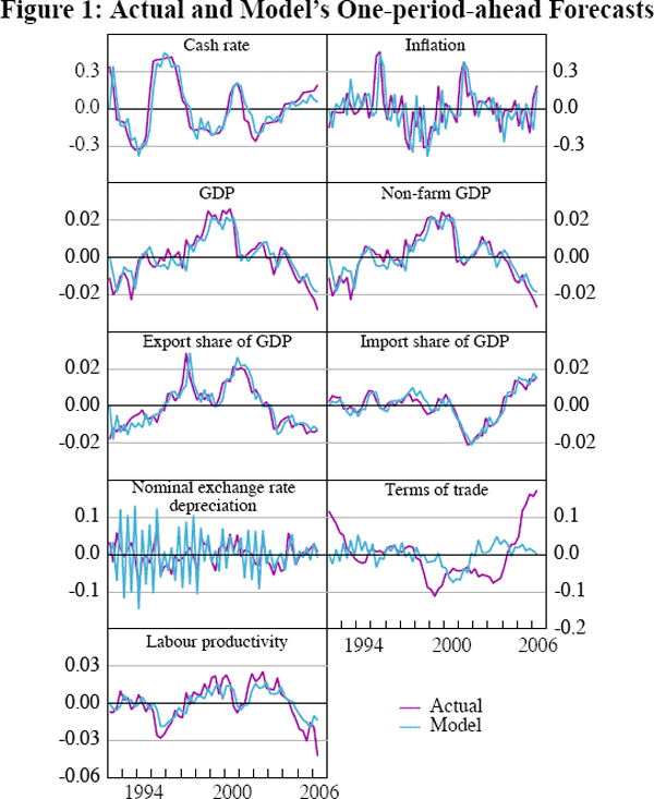
The model provides a very good in-sample description of the dynamics of the cash rate, which is likely to be primarily because its persistence makes it easy to predict. The model is also able to fit most of the other time series reasonably well, with the exception of the terms of trade.
The variances of the errors in the measurement Equation (34) are estimated jointly with the structural parameters of the model. These variances capture series-specific transitory shocks to the observable time series. A low estimated measurement error variance indicates that the associated observable time series matches the corresponding model concept closely. The ratios of the measurement errors over the variance of the corresponding time series are reported in Table 2.
The variance ratios for the various measures of GDP are particularly interesting, since we used multiple indicators for this variable. The estimated values of these ratios indicate that real GDP appears to conform slightly better to the dynamic-and cross-equation implications of the model than real non-farm GDP, but the difference is small. The third indicator for output – domestic market sector GDP – appears to provide the poorest fit.
The terms of trade again stands out as the time series that the model has the biggest problem fitting; the variance of the terms of trade is estimated to be almost entirely due to measurement errors.
4.2 The Open Economy Dimension of the Model
Table 3 below reports the variance decomposition[8] of the model evaluated at the estimated posterior modes reported in Table 1. The first row contains the fraction of the variances that originate from outside Australia. Foreign shocks explain 65 per cent, 67 per cent and 58 per cent respectively of the variance of domestic output, inflation and interest rates. If, instead, a reduced-form VAR(4) in world and domestic output, inflation and interest rates is estimated (with the world variables assumed to be exogenous to the domestic variables), the results suggest that foreign shocks are responsible for 49 per cent, 32 per cent and 45 per cent of the domestic variance of output, inflation and interest rates respectively. The structural model parameterised at the posterior mode thus attributes more of the variance of domestic variables to foreign shocks than the reduced-form regressions; although for output and inflation, the 95 per cent probability intervals include the estimates from the VAR(4).
| Shock/variable | Output | Inflation | Exports | Δ Exchange rate | Interest rate | |
|---|---|---|---|---|---|---|
| y | π | x | Δs | i | ||
| Foreign |  |
0.65 | 0.67 | 0.97 | 0.88 | 0.58 |
| (0.44−0.80) | (0.38−78) | (0.85−1) | (0.76−0.95) | (0.46−0.91) | ||
| Productivity | εa | 0.01 | 0.01 | 0 | 0 | 0 |
| (0−0.16) | (0−0.11) | (0−0) | (0−0.01) | (0−0.01) | ||
| UIP risk premium | εv | 0 | 0 | 0 | 0.01 | 0.01 |
| (0−0) | (0−0) | (0−0) | (0.01−0.01) | (0−0) | ||
| Demand | εy | 0.04 | 0 | 0 | 0 | 0 |
| (0.01−0.19) | (0−0.01) | (0−0) | (0−0) | (0−0.01) | ||
| Cost push | επ | 0.06 | 0.07 | 0 | 0 | 0.04 |
| (0.02−0.15) | (0.04−0.22) | (0−0) | (0−0) | (0.02−0.10) | ||
| Export price | εpx | 0.01 | 0.01 | 0 | 0.01 | 0 |
| (0.01−0.05) | (0−0.04) | (0−0.01) | (0−0.01) | (0−0.03) | ||
| Export demand | εx | 0.21 | 0.23 | 0.03 | 0.10 | 0.24 |
| (0.07−0.33) | (0.12−0.42) | (0.02−0.14) | (0.07−0.16) | (0.11−0.43) | ||
| Import demand | εm | 0 | 0 | 0 | 0 | 0 |
| (0−0) | (0−0) | (0−0) | (0−0) | (0−0) | ||
| Taylor rule | εi | 0.01 | 0.01 | 0 | 0 | 0.02 |
| (0−0.04) | (0−0.03) | (0−0) | (0−0) | (0.01−0.07) | ||
| Note: Figures in brackets indicate 95 per cent posterior probability intervals. | ||||||
The fact that the model can match the reduced-form evidence of the influence of foreign shocks on the Australian economy is reassuring, but is at odds with some previous studies. Justiniano and Preston (2005), using Canadian and US data, find that reduced-form estimates imply that a sizable fraction of domestic volatility does indeed originate abroad. However, their structural model attributes less than 1 per cent to foreign sources. They interpret this as a failure of their structural model to capture the open economy aspects of the data, in spite of its ability to replicate the cross-correlations and dynamics of the Canadian variables.
Apart from the fact that the models are estimated using data for different countries, what can explain this difference in results? One reason may be that Justiano and Preston let the US proxy for the world economy while in this paper the rest of the world is represented by trade-weighted data on a larger set of countries. Any shock that emanates from outside the US, for instance, from Europe, will be attributed to the US in their reduced-form exercise, but it is not clear that a European shock will be appropriately captured by the bilateral US-Canada data.
Another reason why the present model may better capture the impact of foreign shocks is that it is estimated using data on trade volumes. Not using data on imports and exports makes it harder for any model to distinguish between domestic demand shocks and demand for the domestically produced goods coming from abroad.
Table 3 also shows that the model can explain almost all of the nominal exchange rate variance endogenously. The exogenous UIP risk premium shock accounts for only about 1 per cent of the variance of the nominal exchange rate and there is thus less of an exchange rate disconnect puzzle than is found by most other studies.[9]
These results are not significantly affected by the inclusion of measurement errors in some of the time series. Re-estimating the model without measurement errors does increase the posterior mode estimate of the variance of the nominal exchange rate attributable to risk premium shocks, but only to 4 per cent, which is still a much lower figure than that of other studies. Also, the fraction of output variance attributable to foreign shocks falls to 55 per cent and the variance of the interest rate attributable to foreign sources falls to 36 per cent and is thus closer to the reduced-form evidence than the estimated values when measurement errors are included. The fraction of domestic inflation variance attributable to foreign sources increases to over 80 per cent without measurement errors.[10]
The importance of exogenous export demand and income shocks for the dynamics of the model can also be gauged from Table 3. The exogenous export demand shock appears to be more important for explaining output, inflation, the exchange rate and the interest rate than for explaining the variance of exports, which may seem odd at first glance. A possible explanation for this could be that when increased export demand is driven by world developments (which dominates the variance decomposition for exports), imports increase and production for domestic consumption falls. The exogenous demand shock could then be the component of export demand that is not associated with a similar switch of production away from domestic consumption goods. This would lead to the exogenous export demand shock being important for the variance of domestic output, but not very important for the overall variance of exports.
4.3 The Impact of a Monetary Policy Shock
Figure 2 below displays the impulse responses to a unit shock to the (annualised) cash rate for selected endogenous variables together with the 95 per cent highest marginal likelihood intervals.
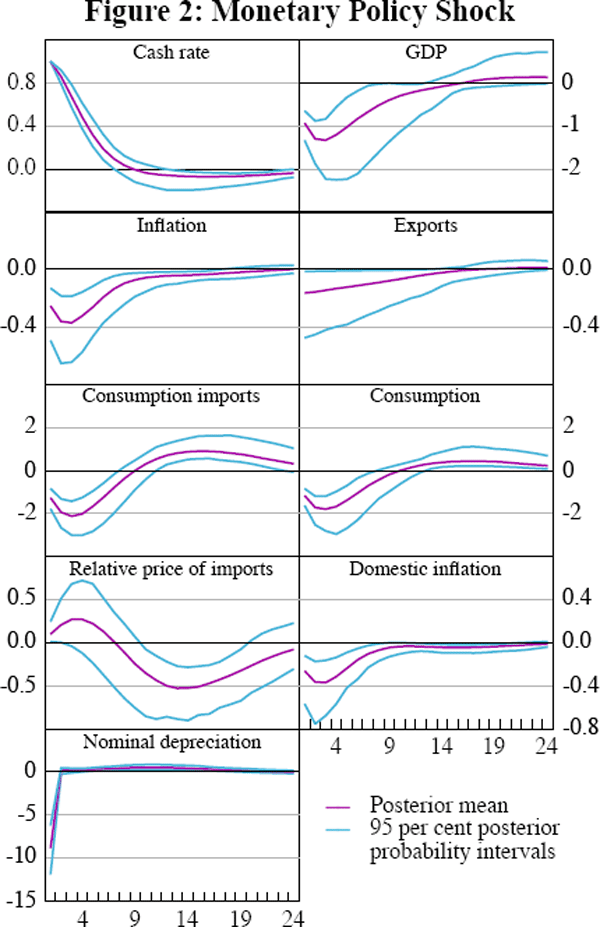
An unanticipated increase in interest rates leads to a fall in output with the maximum negative response of 1.3 percentage points occurring after three quarters. There are two factors contributing to the fall in output. First, the higher real interest rate leads to a fall in domestic consumption. Second, the higher return on domestic bonds leads to a higher demand for the domestic currency denominated assets, leading to a currency appreciation. Lower domestic consumption and less demand for labour both reduce the market real wage, causing a fall in inflation. This is reinforced by the appreciating exchange rate which makes imports cheaper and further decreases inflation. (However, initially consumer prices of imported goods do not fall as much as domestically produced goods, which makes imported goods initially relatively more expensive.) The peak response of (annualised) inflation to the unit shock to the interest rate is a fall of approximately 0.4 percentage points three quarters after impact. The estimated maximum response of output and inflation to a monetary policy shock is faster than that which is found in some other studies, including those employing SVARs.[11] Some of this difference may be explained by the relatively stringent restrictions imposed by the structural model compared to an SVAR. Another factor that could contribute to the relatively rapid response to a monetary policy shock in the present model may be that the sample used does not include the change to an inflation-targeting regime in the early 1990s. If the credibility of the new monetary policy regime was established only gradually, then this could contribute to relatively slow estimated responses of inflation and output to an increase in the cash rate for studies that incorporate this transitory period.
4.4 The Impact of Export Demand and Income Shocks
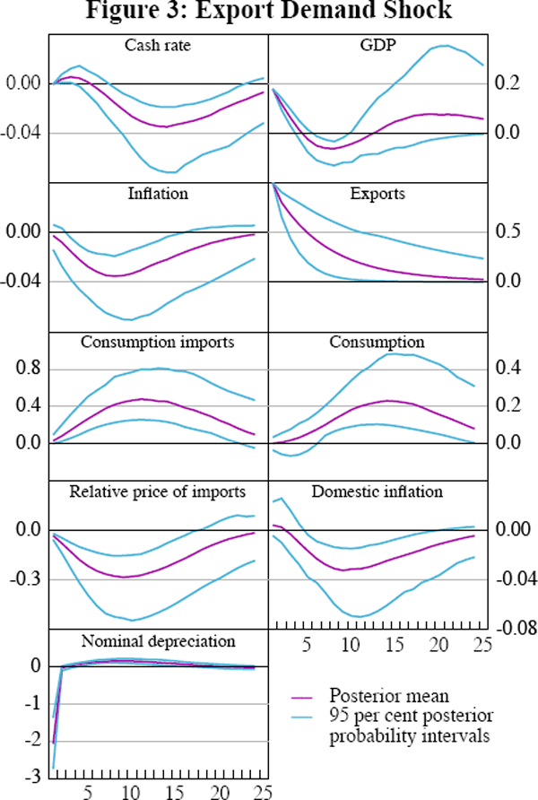
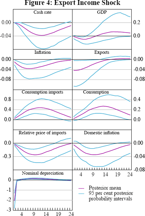
The effects of an exogenous increase in the demand for Australian exports are illustrated in Figure 3. A 1 percentage point increase in export demand leads on impact to a 0.2 percentage point increase in GDP (consistent with the share of the export sector in GDP). It also leads to an appreciation of the exchange rate and boosts imports. The appreciating exchange rate leads to a fall in inflation, though it is quantitatively small (less than 0.03 percentage points at the maximum impact). These effects can be contrasted with the estimated response to a positive shock to the export price. Remember, the main difference between the export price and demand shock is that a price shock does not put direct pressure on the domestic labour market. Figure 4 shows that an income shock, like a demand shock, leads to an appreciation of the exchange rate. The response of the endogenous variables are very similar, with the exception of the volume of exports, which falls due to the appreciating exchange rate. Due to the low elasticity of export demand, the quantitative effect is small.
4.5 The Impact of a Productivity Shock
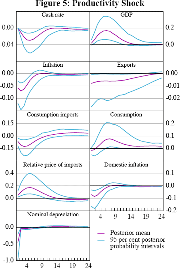
Figure 5 plots the impulse responses to a unit shock to Australian productivity. As expected, GDP increases, inflation falls and the nominal exchange rate appreciates. A less obvious effect is that the consumption of imported goods falls in spite of the appreciating exchange rate. This is because domestic goods prices fall sufficiently so as to make imports relatively more expensive.
Footnotes
The variance decomposition is for the model variables, not the observable time series. For time series that are estimated to contain only a small measurement error component, the numbers in Table 3 are also a relatively accurate approximation to the variance decomposition of the observed times series. [8]
The literature on the exchange rate disconnect puzzle is very large. The seminal paper that defined the ‘puzzle’ is Meese and Rogoff (1983), who showed that exchange rates are very volatile and appear to be disconnected from the macro fundamentals. Examples of recent papers that find a much larger role for the UIP shock are Lubik and Schorfheide (2005) and Lindé et al (2004). [9]
The model without measurement errors was estimated using real GDP as the only indicator for domestic output. More details of the model estimates without measurement errors are available from the author upon request. [10]
See for instance Dungey and Pagan (2000) and Berkelmans (2005). [11]