RDP 2007-11: Global Imbalances and the Global Saving Glut – A Panel Data Assessment 4. Empirical Methodology and Data

Our dataset is an unbalanced panel of annual data for 34 countries over the period 1991–2005, accounting for nearly 90 per cent of global output in 2005. It includes all major economies together with a number of the major oil exporters and those countries directly affected by the Asian crisis.^[3] We choose to explain movements in the current account balance as a per cent of GDP. In contrast to previous studies, for example, those by Chinn and Ito (2007) and Gruber and Kamin (2007), which use five-year average data, our sample comprises annual data.^[4] We do this since annual data may allow us to better identify the impact of financial crises on the current account. In particular, it has the advantage of allowing for short crises whose impact would be muted by the use of five-year averages, and allows a profile for the impact of financial crises on current accounts to be derived.

The independent variables used in this study, which are outlined in greater detail below, can be grouped into two categories: (i) those variables which have traditionally been used to explain movements in the current account; and (ii) variables related to the newer theories that have arisen in response to the widening in the US current account deficit.

Since the sum of the current account balances of the nations in our sample equals zero (ignoring measurement error and assuming the net current account of the small countries excluded from our sample is balanced), a rise in one nation's current account balance must be offset by a fall in the current account balances of other nations. Therefore, a uniform increase in an explanatory variable across all nations should have no effect on the aggregate current account balance of our sample. Accordingly, we have constructed our variables such that the aggregated predicted current account balance is unaffected by a common change in any explanatory variable. To do this, we typically express our explanatory variables as deviations from GDP-weighted averages, consistent with the approach employed by Chinn and Ito (2007) and Gruber and Kamin (2007).^[5]

The data are sourced primarily from cross-country databases, including the IMF's International Financial Statistics (IFS) and the World Economic Outlook (WEO) and the World Bank's World Development Indicators (WDI). For a comprehensive description of the data and its sources, see Appendix A.

4.1 Global Saving Glut and Financial Depth Variables

4.1.1 Financial crises

The global saving glut hypothesis attributes the shift of many developing nations to being net lenders to the ongoing impact of their financial crises. We identify financial crises as those episodes listed as: (i) systemic banking crises in Caprio and Klingebiel (2003); or (ii) a currency crisis lasting for at least 12 months by Kaminsky (2003).^[6] To limit endogeneity problems we exclude those financial crises attributed by Kaminsky to a widening of the current account deficit or sudden stops. Our definition of financial crises is consequently broader than that used by Gruber and Kamin (2007), who only consider systematic banking crises, although our results are not sensitive to using their narrower definition.^[7] We employ some flexibility in the dating of financial crises; we date those which occur late in a year as starting in the following year as they are unlikely to materially affect the annual data until then. A list of crises and their starting dates is presented in Appendix B.

A visual inspection suggests that the increase in the current account balance often peaks about two to three years after a crisis and the effects of crises may be prolonged (Figure 2). However, we also wish to allow the effects of crises to be short if the data dictates. Consequently, we specify financial crises using a dummy variable for the year of the crisis and include a lag for each of the subsequent four years.^[8]

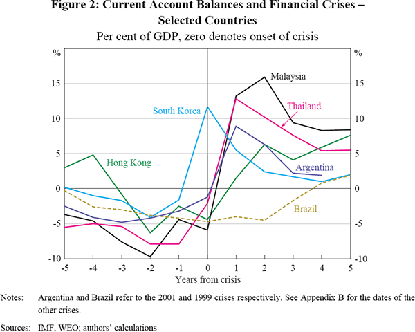
The financial crisis dummies, following Gruber and Kamin (2007), are expressed as deviations from a GDP-weighted average. Consequently, when there has been at least one financial crisis in our sample in a given year, the financial crisis dummy takes on a negative value for those countries that have not had a crisis. The advantage of this approach is that financial crises are allowed to have some (opposite) effect upon the current account balances of nations not in crisis. This is appropriate because the aggregate current account balance of the sample is still zero after each crisis.

4.1.2 Financial depth

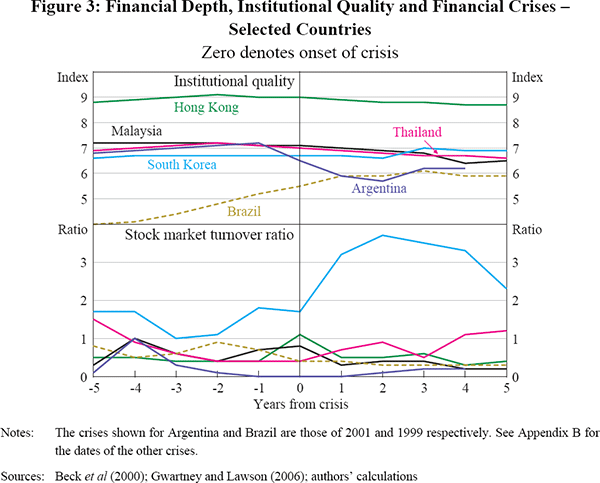
In recent years private capital has flowed into the US and other developed countries. Caballero et al (2007) argue that this is partially because these countries are able to produce suitable financial instruments. We interpret this as meaning that financial markets in these countries are deeper and more liquid. We use annual stock market turnover as a proportion of share market capitalisation (the stock market turnover ratio) from Beck, Demirgüç-Kunt and Levine (2000) as a proxy for financial depth.^[9]

Liquidity is only one dimension of the ‘quality’ of financial assets; for example, the return on an investment also depends on the security of property rights. The quality of institutions in the US and a range of other developed countries may have been a factor contributing to their appeal as a destination for foreign private capital. We measure institutional quality using the Economic Freedom of the World index from Gwartney and Lawson (2006). This index is constructed using five equally weighted sub-indices, including measures of ‘legal structure and property rights’ and the ‘freedom to trade internationally’.^[10] These indices are bounded by zero and ten, with higher values denoting better institutional quality, and are based on both objective and subjective measures. Different measures of institutional quality are used by Chinn and Ito (2007) and Gruber and Kamin (2007). However, we choose the Economic Freedom of the World index because it is readily available and covers a greater range of countries over a longer time period. Movements in the index when financial crises occur are mixed; it does not tend to decline sharply, in part because it is not available at an annual frequency before 2000. Movements in stock market turnover following the onset of a crisis are also mixed, with turnover declining in some instances, but increasing in others (Figure 3).

4.2 Traditional Determinants of the Current Account

The intertemporal model suggests that future economic growth is an important determinant of the current account, and authors such as Engel and Rogers (2006) have argued that the stronger growth prospects for the US compared to other economies, such as in Europe, can explain its current account deficit. In contrast to other recent empirical studies, such as Chinn and Ito (2007), who use the growth rate in labour productivity as a proxy for expected output growth, we use two-year-ahead forecasts from the IMF's World Economic Outlook, which are available for a wide range of countries from 1991 onwards.^[11] These forecasts will include both expected cyclical fluctuations and growth in potential output. Caballero et al (2007) note that:

… it matters a great deal who is growing faster and who is growing slower than the US. If those that compete with the US in asset production (such as Europe) grow slower and those that demand assets (such as emerging Asia and oil producing economies) grow faster, then both factors play in the direction of generating capital flows towards the US. (p 16)

It is difficult to capture such effects in a model such as ours. However, in an attempt to do so we interact the growth forecasts with the three variables that cover various aspects of the perceived depth of a nation's financial markets, namely, stock market depth, the quality of institutions and whether a financial crisis has occurred in the past five years.

To capture the effects of shifts in demographics and in the fiscal position, we include the dependency ratio (the ratio of the non-working-age population to the working-age population) and the fiscal balance as a per cent of GDP.^[12] Growth in the terms of trade (defined as the ratio of export prices to import prices) is included to control for, amongst other things, the effects of fluctuations in global oil and commodity prices on the current account balances of net natural resource exporting countries.

4.3 Estimation

We allow for unobserved time-invariant influences on each country's current account balance by using a fixed-effects estimator. Chinn and Ito (2007) primarily pool data (one constant is estimated for all countries in the sample). The cost of using fixed effects relative to pooling is that we are unable to include variables that are time invariant in the regression. However, time-invariant factors are not a feature of the global saving glut hypothesis, nor Caballero et al's (2007) hypotheses and, therefore, the ability to separately identify them is not of primary concern.

In summary, the regressions we estimate are of the form:

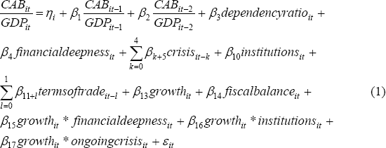
where: η_i is the fixed effect for country i; ε_it the error term; and β_j are parameters.^[13] The model excluding lags of the current account balance is estimated by first differencing Equation (1) to remove the fixed effect and then using Ordinary Least Squares (OLS). When a lag of the dependent variable is included, the first lag of the current account balance will be correlated with the error term, and consequently we use two Stage Least Squares (2SLS), instrumenting the lagged dependent variable with a longer lag. This method is known as the Anderson-Hsiao estimator, after Anderson and Hsiao (1982).^[14] We chose this approach in lieu of using Generalized Method of Moments (GMM), following Arellano and Bond (1991), because our panel has a large time dimension but only a relatively small number of cross-sections. In this case, simulation evidence by Judson and Owen (1999) suggests that the simpler Anderson-Hsiao estimator performs comparatively well in terms of bias.^[15]

Footnotes

The countries included in the data sample are Argentina, Australia, Belgium, Brazil, Canada, China, France, Germany, Hong Kong, India, Indonesia, Iran, Italy, Japan, Kuwait, Malaysia, Mexico, the Netherlands, New Zealand, Nigeria, Norway, the Philippines, Russia, Singapore, South Africa, South Korea, Spain, Switzerland, Taiwan, Thailand, Turkey, the United Kingdom, the United States and Venezuela. [3]

Chinn and Ito (2007) also estimate models based on annual data, however, these are not their primary focus. [4]

The terms of trade is already a relative concept so deviations from GDP-weighted averages were not calculated for this variable. [5]

Crises that Caprio and Klingebiel (2003) date as at least a decade long are excluded (China, Japan and Nigeria), however, their inclusion does not materially change the results. We also require crises in a particular nation to be more than 12 months apart. [6]

Excluding non-banking crises increases the coefficients on the financial crisis dummies, but the results are not changed materially. [7]

In the construction of the lags, we allowed for crises beginning before 1991. Our definition of the financial crisis dummy variables takes into account contagion to the extent that a crisis in one country results in a crisis in another country. [8]

In contrast, Chinn and Ito (2007) use the ratio of private credit to GDP as their proxy variable. We obtain qualitatively similar results using their measure, in lieu of stock market turnover, over a longer sample (1980–2005). [9]

The five sub-indices are: size of government expenditures, taxes and enterprises; legal structure and security of property rights; access to sound money; freedom to trade internationally; and regulation of credit, labour and business. [10]

This compares favourably to other potential sources, such as Consensus Forecasts. Over our sample period, the WEO was published twice a year, in April or May and September or October. We use the April/May forecasts to maximise the forecast horizon. The cost of using these forecasts compared to labour productivity is that they are available for a much shorter time period. Nevertheless, the sample is constrained by the stock market turnover data. [11]

The working-age population is defined as those aged between 15 and 64 years. [12]

We assume that the slope parameters are the same across all countries. Relaxing this assumption is complicated by the need to control for the global current account balance, but would be an interesting area of further research. [13]

The estimation was conducted in Stata 9 using the xtserial and ivreg2 commands for OLS and 2SLS, which are due to Drukker (2003) and Baum, Schaffer and Stillman (2007). [14]

See Roodman (2006) for a discussion of estimating dynamic panels using GMM. Another alternative would be to use the approach of Kiviet (1995), which approximates the size of the bias and corrects for it, and is known as the Least Square Dummy Variable Corrected (LSDVC) estimator. Bruno (2005) generalises this estimator to unbalanced panels. However, it assumes that the explanatory variables are strictly exogenous, which in our case seems to be a strong assumption. [15]