RDP 2008-05: Understanding the Flattening Phillips Curve 4. Has the New-Keynesian Phillips Curve become Flatter?
October 2008
- Download the Paper 318KB
In principle, a correctly-specified new-Keynesian Phillips curve model should not be affected by changes elsewhere in the economy, such as in the policy rule, as it is structural.[10] Also, as these Phillips curves typically rely on direct measures of marginal costs, they should not be affected by any changes in the sensitivity of marginal costs to real activity. Determining whether the estimated new-Keynesian Phillips curve has changed is therefore essential to understanding the likely sources of the instability evident in the reduced-form relationship.
To preview: the results reported in this section suggest that the flattening phenomenon is not limited to reduced-form output-inflation models. Rather, there also seems to have been a change in the linkage between marginal costs (or at least their commonly-used proxy) and inflation. Possible reasons for this breakdown will be explored later, in Section 5.
4.1 Baseline New-Keynesian Phillips Curve Estimates
We estimate the new-Keynesian Phillips curve for the United States using Generalized Method of Moments (GMM) to handle the expectations term, and closely follow Galí, Gertler and Lopez-Salido (2005) and Galí and Gertler (1999).[11] Briefly, assuming that expectations are rational, they will be based on all of the available information, and therefore expectations errors should, on average, be unrelated to the available information (the instruments).[12],[13] In practice, there are several issues with GMM estimation, such as the choice of an appropriate instrument set and lag length to be used in the calculation of robust standard errors and the weighting matrix. Also, when we estimate the deep parameters (for example ω, the share of rule-of-thumb price setters) the model is non-linear, and in this instance the GMM estimates are sensitive to the normalisation used. Many of these issues and their implications for the new-Keynesian Phillips curve are discussed in detail by Guay and Pelgrin (2004), who found that the GMM parameter estimates can be quite sensitive to these modeling choices.
The data we use for the US follow Galí and Gertler (1999). We model the GDP chain price index. The other series (except for the output gap) are for the non-farm business sector. As is standard practice in the literature, real marginal costs are measured using labour's share of income (an assumption which is discussed further in Section 5.2). We use average hourly compensation as a measure of wages, and estimate the output gap using a quadratic trend.
Table 1 presents two sets of estimates of the ‘reduced-form’ hybrid new-Keynesian Phillips curve (Equation (3)) for the United States. Galí and Gertler (1999) refer to this as the reduced form as it does not estimate the deep parameters. The first set of results attempts to replicate the results in Galí et al (2005); it is estimated over the sample 1960:Q1–1997:Q4 and uses real-time data from the St. Louis ALFRED database and their instrument set.[14] These results are indeed very similar, although the standard error for λ, the coefficient on marginal cost, is slightly larger. The second set of results estimates exactly the same regression but using a recent vintage (2007:Q3) of data. Focusing on the estimates of the slope of the Phillips curve, λ, what is stark is that it has reduced by around one-quarter entirely due to data revisions, and its significance has decreased.[15] The estimates over the full sample, (1960:Q1–2007:Q2), however, suggest that the decrease in λ is not entirely due to data revisions.[16] Similar results are obtained if we constrain the coefficients on inflation expectations and lagged inflation to sum to 1 (which implies that β = 1). Pagan (2008) shows that this constraint allows the first lag of inflation to be an instrument for variables other than itself (rather than using deeper lags), which may lessen problems with weak instruments.
| Coefficient | 1960:Q1–1997:Q4 Galí et al (2005) sample |
1960:Q1–2007:Q2 Full sample |
||||||
|---|---|---|---|---|---|---|---|---|
| Real-time data | 2007:Q3 vintage data | 2007:Q3 vintage data | ||||||
| Value |
Standard error |
Value |
Standard error |
Value |
Standard error |
|||
| γb | 0.363 | 0.062 | 0.325 | 0.089 | 0.305 | 0.089 | ||
| γf | 0.630 | 0.058 | 0.661 | 0.084 | 0.689 | 0.087 | ||
| λ | 0.012 | 0.008 | 0.009 | 0.007 | 0.007 | 0.005 | ||
| Imposing γf + γb = 1 | ||||||||
| γb | 0.361 | 0.064 | 0.320 | 0.091 | 0.302 | 0.090 | ||
| λ | 0.011 | 0.006 | 0.007 | 0.006 | 0.006 | 0.004 | ||
| Notes: Estimated using 2SLS with Newey-West standard errors (using 12 lags). Instruments: constant, πt−1 to πt−4, lags 1–2 of the output gap, real marginal costs and nominal wages (following Galí et al 2001). | ||||||||
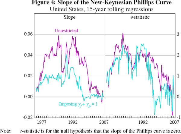
Repeating the rolling regression exercise, but this time for the new-Keynesian Phillips curve, also suggests that a flattening has occurred (Figure 4).[17] Interestingly, compared to the reduced-form estimates, it dates the flattening as having occurred much later, possibly from the early 1990s onwards.

In all, it appears that the flattening of the Phillips curve for the United States may not only be a reduced-form phenomenon.
One approach to try to understand what might have caused this flattening is to look at estimates of the deeper ‘structural’ parameters. Table 2 estimates these over the the entire sample (1960:Q1–2007:Q2) and the sub-samples used in the initial scatterplots of Section 2, namely 1960:Q1–1983:Q4 and 1984:Q1–2007:Q2. Two findings emerge, and these are uniform in direction across the different normalisations and whether or not β is restricted to be 1.[18] First, the Calvo parameter, namely the probability that a firm will be unable to change its price in any given period, appears to have increased, which implies that the average duration between price changes has lengthened considerably. This result adds to the well-known tension between macro-based estimates, such as these, and the much shorter duration between price changes evident from micro data (see Bils and Klenow 2004). Indeed, some of the estimates of the duration between price changes (particularly those from the second moment condition) seem implausibly long. Second, the share of rule-of-thumb firms appears to have decreased. The first finding is consistent with a flattening of the Phillips curve, whereas the second would make it steeper. Overall, it appears the impact of the increase in the Calvo parameter dominates.
| Coefficient | Moment condition 1(a) | Moment condition 2(b) | |||
|---|---|---|---|---|---|
| Value | Standard error | Value | Standard error | ||
| 1960:Q1–1983:Q4 | |||||
| θ | 0.829 | 0.037 | 0.837 | 0.044 | |
| ω | 0.214 | 0.158 | 0.395 | 0.160 | |
| β | 0.999 | 0.051 | 0.994 | 0.056 | |
| Implied λ | 0.022 | 0.013 | |||
| Imposing β = 1 | |||||
| θ | 0.828 | 0.037 | 0.837 | 0.044 | |
| ω | 0.213 | 0.162 | 0.394 | 0.162 | |
| Implied λ | 0.022 | 0.013 | |||
| 1984:Q1–2007:Q2 | |||||
| θ | 0.914 | 0.024 | 0.934 | 0.025 | |
| ω | 0.047 | 0.110 | 0.310 | 0.093 | |
| β | 0.913 | 0.062 | 0.879 | 0.078 | |
| Implied λ | 0.014 | 0.007 | |||
| Imposing β = 1 | |||||
| θ | 0.906 | 0.037 | 0.970 | 0.101 | |
| ω | 0.020 | 0.117 | 0.336 | 0.096 | |
| Implied λ | 0.009 | 0.0005 | |||
| 1960:Q1–2007:Q2 | |||||
| θ | 0.872 | 0.034 | 0.889 | 0.040 | |
| ω | 0.180 | 0.137 | 0.387 | 0.153 | |
| β | 1.000 | 0.036 | 0.984 | 0.040 | |
| Implied λ | 0.013 | 0.007 | |||
| Imposing β = 1 | |||||
| θ | 0.872 | 0.034 | 0.889 | 0.042 | |
| ω | 0.180 | 0.141 | 0.385 | 0.156 | |
| Implied λ | 0.013 | 0.006 | |||
| Notes: (a) Moment condition 1 = E((ϕπt
− θβπt+1 − ωπt−1
− (1 − ω)(1 − θ)(1 −
βθ)mct)zt)
= 0. (b) Moment condition  zt is an element of the time t information set; ϕ ≡ θ + ω[1 − θ(1 − β)]. Estimated using non-linear 2SLS with Newey-West standard errors (using 12 lags). Instruments: constant, πt−1 to πt−4, lags 1–2 of the output gap, real marginal costs and nominal wages (following Galí et al 2001). |
|||||
Another way of trying to gain an intuitive understanding of why this is the case is to look at the data.
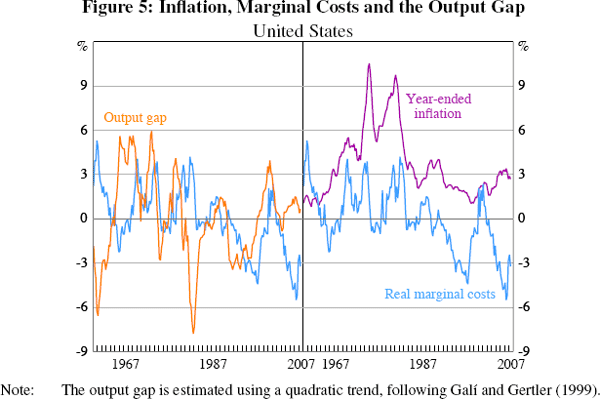
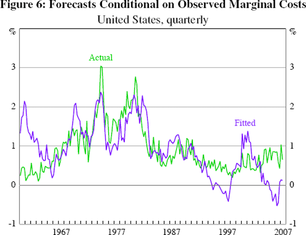
Figure 5 suggests the source of this change: in the United States, at least, there has been a sharp downward trend in labour's share of income since the beginning of the 1990s (the date of the flattening identified by the rolling regressions) or a little earlier, although it is punctuated by a sharp (temporary) upward surge late in the decade.[19] Had inflation responded in the usual way (that is, with the ‘old’ estimate of λ), this would have resulted in a significant trend decline in the inflation rate; instead, inflation fell only modestly over this period (and crept up only slightly in the late 1990s). This is illustrated in Figure 6, which plots a dynamic inflation forecast from the new-Keynesian Phillips curve, conditional on the observed path of marginal costs.[20]


In contrast, an output-gap-based Phillips curve is unlikely to have forecast such subdued inflation, as the gap is estimated to have been broadly around zero over this period (Figure 5). Movements in real marginal costs appear to lag those in the output gap (by approximately one year) and the correlation between them may have decreased over time.[21] However, this could be an artefact of estimating the output gap by de-trending output; in a new-Keynesian model, potential output is typically defined as the level of output that would prevail under flexible prices, and this may not be approximated well by de-trended output, a point emphasised by Neiss and Nelson (2005).[22]
Footnotes
We revisit this in Section 5.4. [10]
Estimates for Australia, which include open economy aspects, are presented in Section 5.2.1. [11]
Galí, Gertler and Lopez-Salido (2001) also instrument real marginal costs, in part, as it may be measured with error, and we do so as well. We also discuss possible data problems in Section 5.1. [12]
The instruments we use include: a constant, lags 1–4 of inflation, lags 1–2 of the output gap, real marginal costs and nominal wages (following Galí et al 2001). [13]
The data are as close to that used by Galí et al (2005) as was possible, but are not identical. The price index is the 1998:Q2 vintage; for the non-farm business sector the first vintage available was 1999:Q3. [14]
The importance of the data vintage has also been noted by Rudd and Whelan (2005) and Guay and Pelgrin (2004). In the context of a conventional, reduced-form specification, Koenig (2003) also found that the significance of unit labour costs was sensitive to data vintage. [15]
Estimates using the 2007:Q3 vintage of the labour share for the whole economy, rather than the non-farm business sector, display a similar decrease in λ. [16]
An obvious caveat to these results is that GMM is a large sample estimator. [17]
They also remain if the sample is split later, for example, in the early 1990s. [18]
Interestingly, as noted by Lawless and Whelan (2007), a comparable downward trend in labour's share is also observed in euro area countries, with a similarly small drop in inflation. [19]
This is the ‘fundamental inflation’ plotted in Galí and Gertler (1999) and Galí et al (2001). [20]
The relationship was also weak during the 1960s (Figure 5). The correlation coefficient between real marginal costs and the output gap for the period 1970:Q1–1983:Q4 is 0.41; it declines to be 0.25 over 1984:Q1–2007:Q2. [21]
In the simplest case, when the representative firm uses labour as the only factor of production, the flexible-price output gap will move proportionally to the marginal cost (see Galí 2008, chapter 3). However, when a more general production function is used, such a simple relationship between the flexible-price output gap and marginal costs may not exist. [22]
