RDP 2011-05: Terms of Trade Shocks: What are They and What Do They Do? 3. Results
December 2011
- Download the Paper 651KB
3.1 Impulse Responses
We follow Peersman (2005) in using a Bayesian approach for estimation and inference and hence capture both sampling and model uncertainty.[4] A total of 100,000 successful draws from the posterior are used to show the median, 84th and 16th percentiles of the impulse responses.[5] Figure 2 shows the accumulated impulse responses of the world variables to the three identified shocks. The direction of these responses (for the first four periods) correspond to the restrictions outlined in Table 1. The magnitudes of these responses, however, are unrestricted. Figure 2 also shows the impulse responses for the terms of trade, which are constructed from the responses of export and import prices.
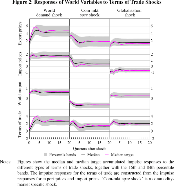
Fry and Pagan (forthcoming) criticise the practise of using the median response as a measure of central tendency because it mixes the responses of different candidate models. They suggest selecting a single model, and hence the unique set of impulse responses from the Monte Carlo draws that is closest to the set of median responses. Accordingly, we also report their ‘median target’ measure. To locate this measure we use the impulse responses from all seven variables in the model.
The responses of variables in the world block to world shocks appear to be permanent. This is consistent with pretesting which indicated that each series was I(1). The effect of each shock on the terms of trade also appears to be permanent, providing additional evidence that export prices and import prices are not cointegrated. Although the magnitudes of the responses of export and import prices to each shock are different, the response of the terms of trade is similar. Each identified shock permanently increases the terms of trade by around 2–4 per cent according to the median target measure.
The response of import prices to the commodity-market specific shock is the only unrestricted response in the world block. The response is clearly positive for the first two quarters, before returning to zero. The response of world output to the commodity-market specific shock is clearly negative. The responses to a commodity-market specific shock are consistent with a textbook ‘commodity supply’ shock, where a disruption to the supply of commodities is followed by an increase in commodity prices, a rise in the price of goods that use those commodities as an input, and a fall in world output. However, without a reliable long-run measure of the world supply of Australia's major export commodities such as coal and iron ore, it is impossible to identify a commodity supply shock.
Figure 3 shows the unrestricted responses of domestic variables to the shocks identified in Table 1. The first column shows the response of the domestic variables to a positive world demand shock. In response to this shock there is a permanent appreciation in the real exchange rate of 2–3 per cent. The median impulse response suggests that level of output is 0.25 per cent higher for three quarters, although the median target measure suggests a somewhat weaker response. Nominal interest rates increase by about 50 basis points and remain elevated for around two years. Inflation is slightly higher on impact (due to higher import prices), but rapidly returns to zero as the exchange rate appreciates and the interest rate increases.
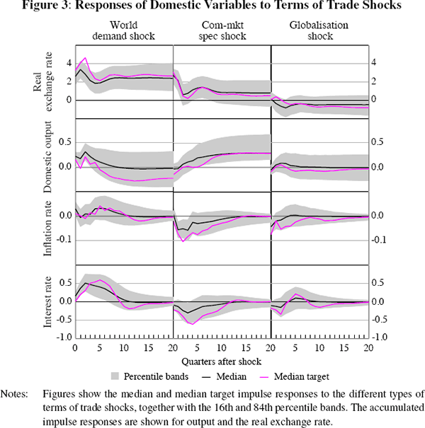
The central column of Figure 3 contains the responses to a commodity-market specific shock. In response to this shock, the real exchange rate appreciates by around 3 per cent on impact and then depreciates by the same amount over the next three quarters. The higher real exchange rate appears to be passed through to lower consumer prices for three quarters after the shock, although the magnitude of the inflation response is small (less than 0.1 per cent per quarter). This suggests that any domestic inflationary pressures that might arise from the higher import prices are offset by the higher real exchange rate, and the interest rate falls accordingly. According to the median and median target, the level of domestic output is permanently higher following a commodity-market specific shock, however the strength of this response is imprecisely measured, with the 16th percentile band touching zero.
The last column of Figure 3 shows the response of the domestic variables to a positive globalisation shock. In this case the real exchange rate appears to depreciate, although the estimated magnitude of this depreciation is small. Although it may be surprising to see the real exchange rate depreciate in response to a positive shock to commodity prices, this response is consistent with a Balassa–Samuelson type effect. Domestic inflation falls on impact before returning to trend in 4 to 8 quarters, perhaps due to the depreciation of the real exchange rate. There is no significant response by the short-term nominal interest rate or output.
To summarise, the evidence presented here is that terms of trade shocks are not necessarily expansionary or inflationary, with the net effect dependent upon the nature of the underlying shock. The real exchange rate appears to have provided an important buffer against foreign shocks over the sample period. Overall, monetary policy – as captured by the short-term market interest rate – has tended to respond to the foreign shocks in such a way that it reduces the inflationary effect of these shocks.
3.2 Variance Decomposition
Table 2 reports the contribution of the three identified shocks to the unconditional variance of the data. We report the results for the median target draw, rather than the median because the construction of variance, and historical, decompositions requires that shocks come from a unique model. We also examined variance decompositions at shorter horizons, but the results were broadly similar and are not reported here.
| πx | πm | Δyw | Δq | Δyd | πd | rd | |
|---|---|---|---|---|---|---|---|
| World demand shock | |||||||
| Median target | 43 | 36 | 68 | 39 | 20 | 3 | 18 |
| One std dev interval | (21,51) | (19,55) | (35,75) | (15,41) | (9,23) | (2,16) | (4,26) |
| Commodity-market specific shock | |||||||
| Median target | 51 | 45 | 16 | 36 | 6 | 18 | 18 |
| One std dev interval | (39,68) | (29,66) | (10,39) | (18,45) | (4,14) | (3,17) | (2,16) |
| Globalisation shock | |||||||
| Median target | 6 | 19 | 15 | 1 | 3 | 6 | 4 |
| One std dev interval | (4,17) | (7,24) | (5,37) | (3,11) | (3,12) | (1,10) | (1,10) |
| Shocks to domestic block | |||||||
| Median target | 24 | 70 | 73 | 59 | |||
| One std dev interval | (24,39) | (59,76) | (63,87) | (57,84) | |||
The variance decomposition indicates that the commodity-market specific shock and the world demand shock account for the largest share of the variance in the world price of Australian exports (51 percent and 43 per cent, respectively) and imports (45 per cent and 36 per cent, respectively). The globalisation shock appears to be less important but notably has a larger impact on Australian import prices: the median target measure suggests that the globalisation shock accounts for 6 per cent of the variance in export prices and 19 per cent of the variance in import prices. Most of the sample variation in world output growth is attributed to the world demand shock (68 per cent), with roughly similar contributions from the commodity-market specific shock (16 per cent) and the globalisation shock (15 per cent).
The variance decomposition can also be used to quantify the extent to which the floating exchange rate has provided a shock absorbing mechanism against global shocks. If the exchange rate effectively stabilises foreign shocks, then these shocks should have a substantial effect on the exchange rate, but much less of an impact on the other domestic variables. Table 2 shows that the variance of the real exchange rate is explained predominantly by the world shocks, with the median target draw indicating that only 24 per cent of variation in the real exchange rate is explained by ‘domestic’ factors.[6] Other unidentified shocks explain substantially more of the variation in the remaining domestic variables. According to the median target measure, 70 per cent of the variance in domestic output and 73 per cent of the variance in trimmed-mean inflation is explained by domestic factors. These results indicate that the exchange rate does indeed provide an important buffer against the force of global shocks.
3.3 Historical Decomposition
Historical decompositions can be used to estimate the contribution of the identified shocks to each variable in the model over time. Figure 4 shows the contributions of each shock to quarterly growth in export prices and import prices variables over the sample period using the median target measure.
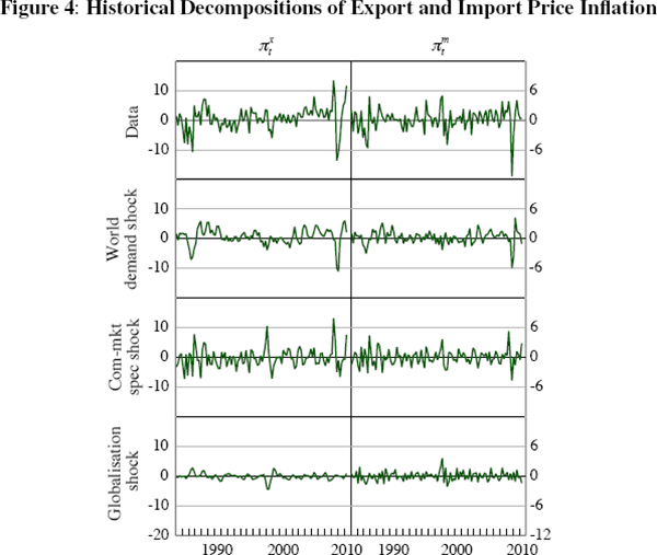
Export prices appear to have been subject to several sizeable commodity-market specific shocks throughout the sample period, most notably in mid 2008. The commodity-market specific shock appears to be coinciding with a shift in the composition of world growth in the first half of 2008. Although major trading partner growth fell well below the sample average in the June quarter of 2008, Chinese GDP growth remained a little higher than the sample average, though a sluggish supply response may also have contributed to the run-up in commodity prices.[7]
The decline in export prices that followed in late 2008 is, unsurprisingly, explained by a negative world demand shock and subsequent recovery is attributed mainly to a commodity-market specific shock. The recovery broadly coincides with the Chinese fiscal stimulus, which had a strong emphasis on infrastructure projects. Although the globalisation shock explains a relatively small proportion of the variation of export prices, it is estimated to have contributed to the decline – and the subsequent increase – in export prices during the Asian financial crisis in the late 1990s.
Figure 5 shows the contributions of each shock to quarterly growth in world output and the terms of trade. The decline in world output growth during the Asian financial crisis is explained by the combined effects of a negative globalisation shock and a negative commodity-market specific shock. In contrast, the sharp decline in world output in late 2008 and early 2009 is explained by a negative world demand shock with a smaller contribution from a commodity-market specific shock.
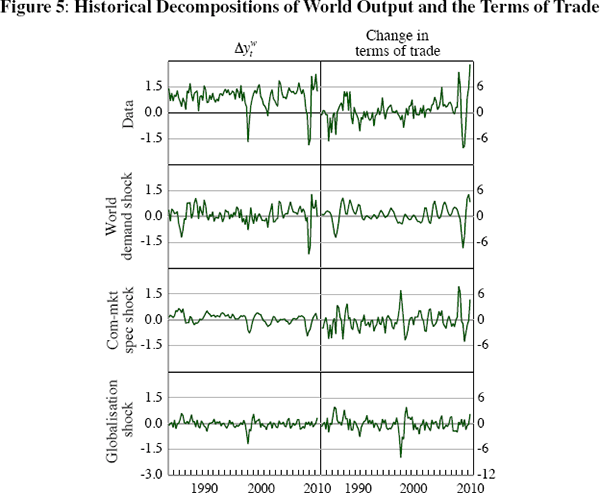
Figure 6 plots the contribution of terms of trade and ‘domestic’ shocks to quarterly growth in the real exchange rate and domestic output and Figure 7 plots the contribution of these shocks to quarterly inflation and the interest rate. Fluctuations in the real exchange rate are explained by a combination of global and domestic shocks, with a very limited role for the globalisation shock.
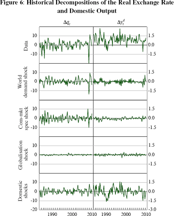
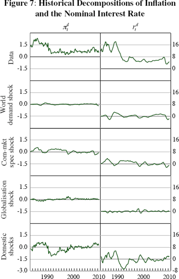
The world shocks appear to have made only modest contributions to historical variations in output, inflation, and short-term interest rates. However, a significant proportion of the late 2008 contraction in real GDP growth, and much of the subsequent recovery, is attributed to the combined effects of a negative world demand shock and domestic shocks. This contrasts with the recession of the early 1990s, which the sign-restricted VAR attributes almost entirely to shocks to the domestic block.
3.4 Additional Results and Robustness Checks
3.4.1 Estimation over the inflation-targeting period
As a robustness check, we estimated the benchmark VAR over the inflation-targeting period. The estimated impulse responses are broadly similar, although the one-standard deviation error bands are wider in some cases (see Figures B1 and B2). The variance decomposition is qualitatively similar to the longer sample (see Table B1).
The historical decompositions are shown in Figures B3, B4, B5 and B6. When the model is estimated over the inflation-targeting period, the commodity-market specific shock appears to be somewhat more important for explaining the variation in import prices, world output, and the real exchange rate, and the world demand shock appears to be less important than in the longer sample. Moreover, global shocks are estimated to explain a greater proportion of the variation in interest rates. Of the global shocks, the globalisation shock is estimated to be more important in accounting for variation in inflation while the world demand shock and the commodity-market specific shock explain more of the variation in interest rates.
3.4.2 Direct versus indirect effects on inflation
The consumer price index captures the prices of both tradable and non-tradable goods. Terms of trade shocks will have a direct impact on CPI inflation via the price of tradable goods but there can be indirect (second round) effects as well. To evaluate the relative importance of direct and indirect effects on inflation, we extend the domestic block of the benchmark VAR to include both non-tradable and tradable inflation in place of trimmed-mean inflation.
The impulse responses of tradable and non-tradable inflation to the three global shocks are shown in Figure 8. The impulse responses of the remaining variables in the extended VAR are similar to those presented for the benchmark VAR in Figure 3 and are not shown.
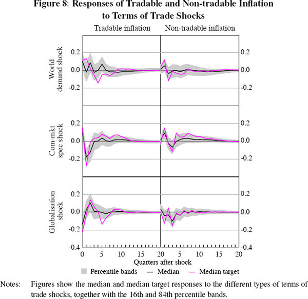
The world demand shock has very little impact upon tradable or non-tradable inflation, consistent with the results for trimmed-mean inflation shown in Figure 3. For the commodity-market specific shock, the negative response of consumer price inflation appears to be mainly driven by the response of the tradable component, which is slightly offset by the positive response from the non-tradables component. Inflation is initially lower after a globalisation shock. Figure 8 indicates that this is likely to be due to the decline in tradable inflation. However, tradable inflation rises in subsequent periods, perhaps due to the depreciation of the real exchange rate. The effect of this increase on trimmed-mean inflation is, however, offset by a modest decline in non-tradable inflation.
The variance decompositions for non-tradable and tradable inflation are shown in the last two columns of Table 3. We do not show the variance decomposition for the world block as this is identical to results presented in Table 2. Not surprisingly, domestic shocks explain a larger share of non-tradable inflation than tradable inflation. This provides further evidence that the floating exchange rate has provided an effective buffer to external shocks.
| Δq | Δyd | rd | πnt | πt | |
|---|---|---|---|---|---|
| World demand shock | |||||
| Median target | 22 | 30 | 13 | 6 | 9 |
| One std dev interval | (18,43) | (8,20) | (3,20) | (4,13) | (5,14) |
| Commodity-market specific shock | |||||
| Median target | 44 | 8 | 11 | 13 | 18 |
| One std dev interval | (15,41) | (4,13) | (2,13) | (4,14) | (6,17) |
| Globalisation shock | |||||
| Median target | 3 | 3 | 4 | 8 | 13 |
| One std dev interval | (3,11) | (4,11) | (2,11) | (3,12) | (4,12) |
| Shocks to domestic block | |||||
| Median target | 31 | 60 | 72 | 73 | 60 |
| One std dev interval | (27,41) | (62,78) | (63,85) | (67,83) | (62,78) |
| Notes: Results for the world block are unchanged from Table 2 and are not repeated here; πnt is non-tradable inflation and πt is tradable inflation | |||||
Footnotes
Detailed descriptions of algorithms used for Bayesian inference in these models can be found in Peersman (2005), Uhlig (2005), and Rubio-Ramírez, Waggoner and Zha (2010). [4]
Because the point-wise distribution of each impulse response is approximately normal, the 16th and 84th percentiles roughly correspond to a one standard deviation error band. [5]
We are cautious in the use of the word ‘domestic’ in this situation because own shocks to the real exchange rate may not be entirely domestic in origin. For example, global risk-premia shocks are often cited as important sources of variation in the exchange rate [6]
Annual data from ABARES and the US Geological Survey suggest that growth in the world supply of some commodities, such as iron ore, slowed sharply in 2007 and 2008. [7]