RDP 2012-01: Co-movement in Inflation 4. Results
March 2012 – ISSN 1320-7229 (Print), ISSN 1448-5109 (Online)
- Download the Paper 814KB
This section presents the key results from the panel VAR model. First, we document that co-movement in inflation is an important feature of the G7 data, even after controlling for domestic economic activity and common movements in real activity and commodity prices. Second, we investigate which of the key potential drivers of inflation in the model (in particular, the common indicators of real activity and commodity prices) are most important for driving inflation co-movement.
4.1 Co-movement in G7 Inflation
As discussed in the previous section, the common inflation indicator included in
the panel VAR was constructed giving equal weight to the two lags of (standardised
and de-meaned) quarterly CPI inflation ( )
for all (n = 7) countries. The indicator was included in each country's
inflation equation in the panel VAR, and with the same coefficient. The indicator
is described in Equation (2):
Where  represents the estimated posterior distribution of the factor loading. There would
be evidence in favour of co-movement in inflation being an important feature
of the data if
  is estimated quite precisely and centred
away from zero. Or, to put it another way, a significant factor loading would
suggest that lags of other country's inflation rates (that is, information
on foreign inflation) is a useful explanator of domestic inflation.
Figure 2 plots the median, 5th and 95th percentile of the estimated posterior distribution
of the common inflation indicator ( ).[10]
The figure highlights the common nature of inflation experiences, with inflation
rates in the individual G7 countries typically either above or below their
respective historical averages at the same time. Further, the posterior distribution
of the common inflation indicator is estimated quite tightly and is centred
away from
zero.[11]
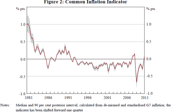
This result suggests that movements in foreign inflation have explanatory power for domestic inflation in the G7, even after controlling for other potentially important features of the data. As highlighted earlier, indicators capturing co-movement in real activity and common commodity price movements, along with country-specific factors (including lagged domestic inflation), were also included in the panel VAR.[12]
Another way to analyse ‘global inflation’ dynamics in the panel VAR is to consider the effect of ‘shocking’ different inflation equations. While it is difficult to identify structural shocks in our setting (for example, ‘orthogonalised’ impulse response functions would require a particular ordering of countries and variables which seems difficult to justify using theory), generalised impulse response functions (GIRFs) (see Koop, Pesaran and Potter (1996) and Pesaran and Shin (1998)) can be constructed that are independent of the ordering of variables and countries. GIRFs consider the effect of a shock (or subset of shocks) to a particular equation (or subset of equations) and integrate out the effect of other shocks according to their historical distribution (we assume the errors follow a multivariate normal distribution). While GIRFs cannot be given a clear structural interpretation, they are informative about the key dynamics of the model and are useful to describe how shocks to different equations evolve through the system.
Figure 3 shows GIRFs of a one standard deviation shock to the US inflation equation in the panel VAR.[13] The median response on domestic inflation in each of the G7 economies over 20 quarters is shown in the left-hand panel, with the median response in the other G7 economies as a whole (average of the G7 excluding the United States) and 90 per cent posterior probability interval shown in the right-hand panel. In the figure, inflation has been re-scaled using the standard deviation of each series (to correspond to actual units) and is presented as an annualised rate.
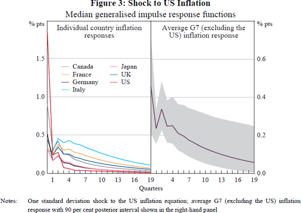
A one standard deviation shock to the US inflation equation in the panel VAR corresponds to an increase in inflation in the United States of around 1¾ percentage points (in annual terms). The shock coincides with a synchronised increase in inflation in the other G7 countries of between 0.3 and 0.9 percentage points on impact. The average response to inflation across countries (excluding the US) is around 0.45 percentage points, with the bulk of the posterior distribution away from zero. The shock is also quite persistent, with inflation at least 0.15 percentage points higher in the other G7 countries, on average, up to two years after the initial shock. These results again highlight the significant cross-country co-movement between inflation rates in the G7. We now turn to discuss the potential drivers of this co-movement.
4.2 What is Driving the Co-movement in G7 Inflation?
4.2.1 Co-movement in real activity
As discussed in Section 3, a common real activity indicator was
included in the panel VAR, designed to capture co-movement in real variables
across the G7. It was constructed giving equal weight to two lags
each of (standardised and de-meaned) output, consumption and investment
growth for all countries. The indicator was allowed to load separately in real
variable equations, with coefficient  (Equation (3a)), and
inflation equations, with coefficient
  (Equation (3b)).
To investigate the significance of this indicator for explaining movements in both
real activity and inflation across the G7, Figure 4 plots the median, 5th and 95th percentile of the estimated posterior distribution
of the common real activity indicators,  (top panel) and
  (bottom panel).
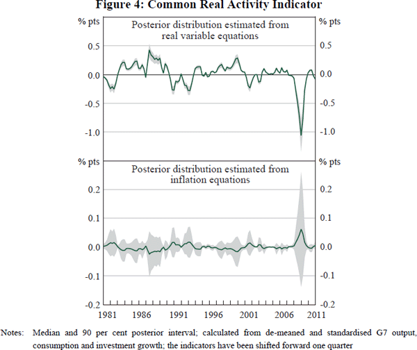
Looking at the top panel of Figure 4, common influences were found to be an important driver of real variables in the data. When the common real activity indicator was included in each of the output, consumption and investment growth equations, the posterior distribution was estimated quite precisely and centred away from zero. This result is consistent with other results in the literature (for example, Kose et al (2003) and Canova et al (2007)) which find that a common factor can explain a substantial share of variation in real variables across countries.
In contrast, co-movement in real activity is not significant in driving fluctuations in inflation across G7 countries. As shown in the bottom panel of Figure 4, the 90 per cent posterior interval of the common real activity indicator includes zero for most of the sample, with the median estimate of the factor loading slightly negative. We can also use GIRFs to investigate the significance of correlated movements in real activity for inflation in the panel VAR. Figure 5 presents GIRFs of inflation to a ‘common’ shock to real activity, defined as a one standard deviation shock to a subset of equations – output, consumption and investment – for all countries in the panel VAR.[14] On impact, the positive shock increases output, consumption and investment by, on average across countries, around 0.35, 0.25 and 0.75 per cent, respectively. The median individual country inflation responses to this shock are shown in the left-hand panel of Figure 5, with the median response for inflation in the G7 as a whole (calculated as the average across countries) and 90 per cent posterior probability interval shown in the right-hand panel.
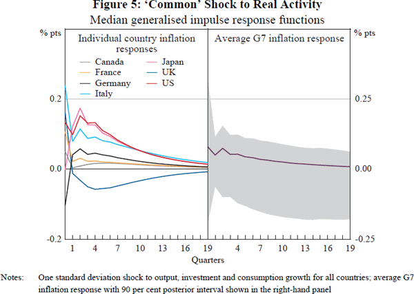
The results suggest that the ‘common’ positive shock to real activity, as characterised here, does increase inflation in some countries but by a modest amount, with the response across countries less synchronised than was the case following the shock to US inflation (Figure 3). The 90 per cent posterior band for the average G7 inflation response is also relatively wide and includes zero (this is also the case for the individual country responses).
Correlated movements in real activity, therefore, do not seem to be a significant driver of G7 inflation in the panel VAR. A possible reason for this finding is that a reasonable part of our estimation sample from 1981:Q2 to 2011:Q1 is comprised of the ‘great moderation’, a period that has seen a reduction in the variability of both real activity and inflation. Given this, it may be harder to precisely estimate the relationship between these variables. It has also been argued that this period has seen a substantial ‘flattening’ of the Phillips curve (see, among others, Beaudry and Doyle (2000) and Roberts (2006)), with inflation less responsive to changes in output. It is also worth emphasising again that generalised impulse responses cannot be given a clear structural interpretation. Given that the ‘common shock to real activity’ characterised above could reflect both demand and supply shocks (which would have opposite effects on inflation) this may also be a reason for the muted estimated inflation response.
Another important point is that the correlations we are interested in are likely to be unstable over time. One limitation of our analysis is that we do not allow for time variation in the parameters of the model. It could be the case that common movements in real activity are more important at particular times. For example, the synchronised fall in economic activity experienced following the global financial crisis (see Figure 4, top panel) was associated with a synchronised fall in inflation across countries (see Figure 2). During this particular period, synchronised movements in real activity could have been an important driver of this inflation co-movement. Non-linear effects are also not considered here (see Stock and Watson (2010) for further discussion on the stability of inflation forecasting models, particularly during downturns).
Nevertheless, overall these results would suggest that we need to look elsewhere to explain the observed co-movement in inflation rates seen in the data.
4.2.2 Common shocks to commodity prices
As discussed in Section 3, oil and non-fuel commodity prices were included as exogenous variables in the panel VAR as a way to control for particular common shocks to which all countries are exposed. The simple average of contemporaneous and lagged oil price inflation was found to be a significant explanator of inflation in the panel VAR. The median coefficient estimate was positive, with the 90 per cent posterior probability interval away from zero. The median coefficient estimate in the panel VAR implies that a 10 per cent shock to oil prices increases headline inflation in the G7 by, on average across countries, around 0.2 percentage points in annual terms in the same period. The non-fuel commodity price variable was also found to be important for explaining inflation (the contemporaneous inflation response to a 10 per cent increase in non-fuel commodity prices in the panel VAR was, on average across countries, around 0.2 percentage points). For the real activity variables in the panel VAR, non-fuel commodity prices, but not oil prices, were found to be a significant explanator.
Commodity prices therefore seem to be an important driver of headline inflation across countries, which could go some way to explaining the observed co-movement in inflation rates observed in the data. The assumption that commodity prices are exogenous to the other variables in the panel VAR, however, is perhaps too restrictive and could lead to biased estimates of the contemporaneous impact of commodity prices on inflation. For example, common movements in real activity (reflected in the common real activity indicator in the panel VAR) could influence global commodity demand and therefore commodity prices. Therefore, to check this result, an alternative specification was also estimated in which commodity prices are endogenously determined in the panel VAR. In particular, the oil and non-fuel commodity price inflation variables were assumed to be explained by lags of each other, but also by the common real activity and common inflation indicators included in the panel VAR. Figure 6 presents GIRFs of a 10 per cent shock to oil prices on inflation in the G7 under this alternative specification.[15]
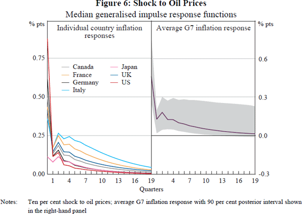
The GIRFs reported in Figure 6 again support the idea that common shocks to commodity prices are a key candidate for explaining the observed co-movement in headline inflation in the G7. The shock to the oil price equation in the panel VAR leads to a synchronised increase in inflation across the G7, with inflation initially increasing by between 0.1 and 0.9 percentage points across countries and by 0.45 percentage points on average (with the 90 per cent posterior probability interval away from zero for up to two years after the shock). Under this alternate specification, with commodity prices allowed to be endogenous, a shock to non-fuel commodity prices was also found to have a significant impact on inflation (although part of this is due to the fact that movements in non-fuel commodity prices have historically been associated with an increase in oil prices and GIRFs are not ‘orthogonalised’).
Another way to consider the role of commodity prices in driving global inflation dynamics is to model consumer prices excluding food and energy; that is, core, rather than headline, inflation. By removing food and energy price movements from the headline measure we strip out the direct first-round impact of shocks to food and energy prices on consumer prices. If movements in these variables are indeed an important driver of the significant correlation between headline G7 inflation rates, we would expect to see less evidence of core inflation moving together across countries. Figure 7 presents the common inflation indicator from the panel VAR model estimated using core, rather than headline, inflation, while Figure 8 shows GIRFs of a one standard deviation shock to the US core inflation equation.
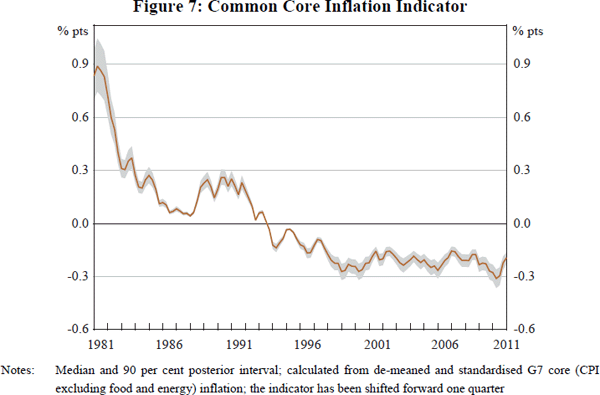
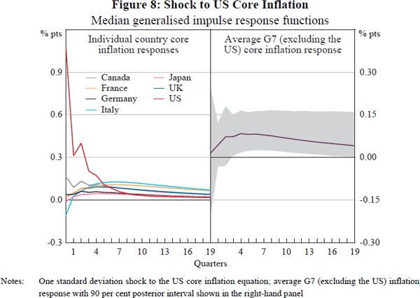
As can be seen in Figure 7, the estimated loading on the common core inflation indicator was still found to be positive and estimated quite precisely, suggesting that there is also evidence of co-movement in core inflation rates being an important feature of the data. In contrast to the panel VAR estimated using headline inflation, however, the contemporaneous impact of a shock to US core inflation on the rest of the G7 (Figure 8) is close to zero and insignificant (the peak response is lagged by around a year and although the 90 per cent posterior probability interval is slightly away from zero further out, the magnitude of the average response remains relatively small). So while there is still evidence of co-movement in core inflation rates in the G7, it is perhaps somewhat less pronounced than in the headline data. This seems consistent with the notion of common shocks to commodity prices being an important determinant of inflation co-movement.
4.3 Robustness
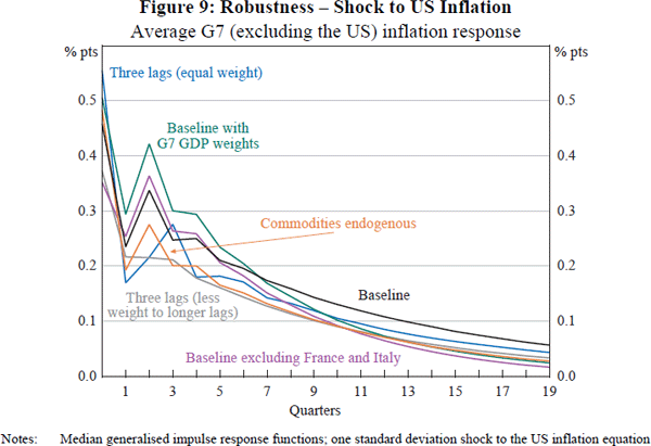
A number of different specifications of the panel VAR model outlined above were estimated to check the robustness of the results. In particular, versions of the model were tried using different lag lengths and also giving declining weight to longer lags when constructing the various indicators. Country weights corresponding to GDP at market exchange rates (on average over the sample) were also tried as opposed to giving equal weight to each country. A version of the model excluding France and Italy was also estimated to see whether including multiple European countries (with the same exchange rate for part of the sample) was influencing the results. And as mentioned above, a version of the model where commodity prices are endogenously determined was also estimated. The results were generally found to be robust to these alternate specifications. For example, Figure 9 plots the average G7 (excluding the United States) inflation GIRF to a US inflation shock (the same shock shown in Figure 3) under different specifications of the panel VAR.
The baseline panel VAR was also estimated over a more recent ‘low-inflation’ sample from 1992:Q1 to 2011:Q1, using a prior initialised over the earlier sample period. This is important to consider since the policy shift towards inflation targeting around the early 1990s is potentially a key regime change in our sample. The transition from a period of relatively high and volatile inflation to lower and more stable inflation in the early 1990s was common to each of the G7 economies. From a purely statistical point of view, the co-movement in inflation rates around this time could be a key driver of the global inflation result. The posterior distribution of the common inflation indicator (both the headline and core version) estimated over this ‘low-inflation’ sample is shown in Figure 10. While estimated somewhat less precisely relative to the full sample, the indicators were still found to be an important explanator of domestic inflation in the panel VAR. This would suggest that the shift to low inflation cannot account for all of the co-movement in inflation rates observed in the data.
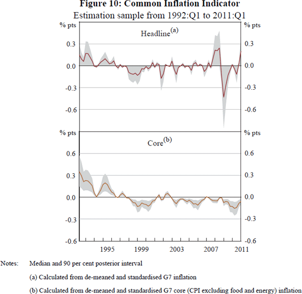
Finally, a version of the panel VAR was also estimated in which the factorisation of the coefficients (essentially restrictions) described earlier was not assumed to be exact (see Appendix A). The results obtained were again similar to those reported above. We also estimated the model using feasible least squares and calculated robust standard errors as an additional robustness check. Again the results were similar (see Appendix B).
Footnotes
The units of Figure 2 should be interpreted in terms of quarterly de-meaned and standardised inflation. The mean quarterly inflation rate for the G7 countries over the sample is 0.75 per cent, with an average standard deviation of 0.7 per cent. [10]
The fact that the posterior uncertainty bands ‘shrink’ when the indicator is close to zero is a result of the (de-meaned and standardised) inflation data itself being close to zero in certain periods. The posterior uncertainty surrounding the estimated factor loading, however, remains constant throughout. [11]
The real country-specific indicators were found to be important drivers of real variables for all countries except for Japan, and offered some explanatory power for inflation in the United States, Japan, Germany and the United Kingdom. The country-specific inflation indicators (lags of domestic inflation) were found to be important in all of the inflation equations, and also the real variable equations for the United States, Japan and Canada in particular. We found less evidence of variable-specific effects being important for output, consumption or investment. These results are available on request. [12]
The United States was not chosen for any particular reason here and the GIRFs look similar if a different country's inflation equation is shocked instead. [13]
See Koop et al (1996) and Dees et al (2007) for a discussion of how a subset of system-wide shocks can be analysed in the generalised impulse response framework. [14]
It is also worth noting that in the specification with commodity prices endogenously determined, we do not restrict the contemporaneous impact of oil prices to be the same across countries (as is the case when commodity prices are assumed exogenous and enter the model contemporaneously and with the same coefficient across countries). [15]

