RDP 2012-02: The Role of Credit Supply in the Australian Economy 5. Results

The model is estimated using quarterly data over the period December 1983 to December 2011. Confidence bands are generated using a Monte Carlo procedure.^[23]

5.1 Response to a Credit Supply Shock

As discussed, the survey measure of the difficulty obtaining finance is assumed to primarily reflect credit supply dynamics. Hence, we identify credit supply shocks as the orthogonal innovations in this series. Credit shocks may also operate in part through the spread variable, although, as already noted, this is poorly measured and may also capture demand shocks. Figure 7 illustrates estimated impulse responses to a one standard deviation shock to the difficulty of obtaining finance – that is, a 5½ percentage point increase in the balance of firms reporting greater difficulty obtaining finance.

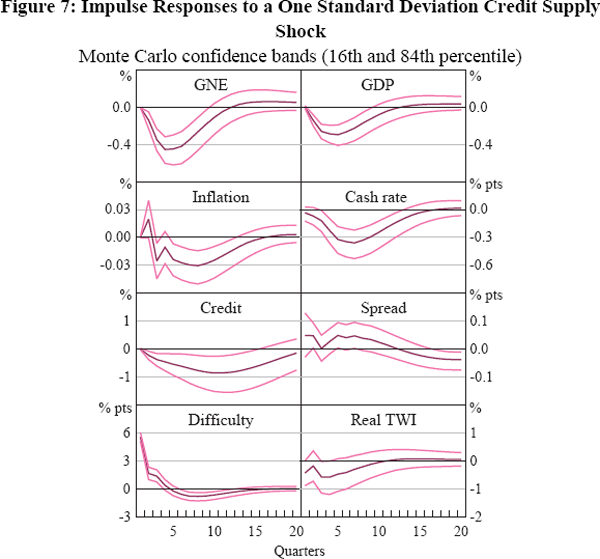
These results suggest that credit supply shocks have a significant effect on the real economy. Australian GDP is nearly ⅓ per cent lower one year after the initial shock and then starts to gradually increase back to its baseline level. Interestingly, the decline in GNE is much larger than the decline in GDP (nearly ½ per cent); this suggests that net exports make a positive contribution to GDP growth after a credit supply shock, in line with the depreciation of the real exchange rate. There is also a decline in business credit, which is larger and more persistent than the fall in output – it takes two and a half years for business credit to reach a trough following a credit supply shock, falling by nearly 1 per cent relative to its baseline. Credit spreads increase after the credit shock, although the magnitude of the increase is small (under 10 basis points). The cash rate declines by 0.4 percentage points after 18 months, before gradually reverting back to baseline. This could reflect both an indirect response to the macroeconomic effects of the shock and possibly a direct policy response to the tightening in credit supply.

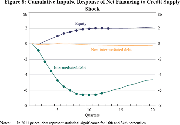
While the results indicate that a credit shock produces a fall in intermediated business credit, firms might react to the shock by tapping other sources of finance such as bonds or equity. To examine this possibility we make use of an alternative dataset of external funding by non-financial businesses separated into equity, non-intermediated debt (i.e. bonds) and intermediated debt (i.e. credit). These data are available from 1986. The results show that the fall in business credit is partly offset by a persistent increase in equity, as firms look to rebuild their balance sheets (Figure 8). However, there is little offset from an increase in non-intermediated debt, suggesting that much of the decline in business credit is due to bank-reliant firms with little recourse to the bond market.

5.2 The Historical Importance of Credit Supply Shocks

A decomposition of structural VAR forecast errors can provide a measure of the importance of shocks during different historical episodes. Figure 9 shows the contribution of credit supply shocks to GDP forecast errors over time. During the global financial crisis, credit supply shocks contributed to weaker GDP from mid 2007, with GDP furthest from the model's forecast in June 2009 (by −1 per cent). This was one of the largest deviations of GDP from baseline due to a credit supply shock in the model's history.^[24]

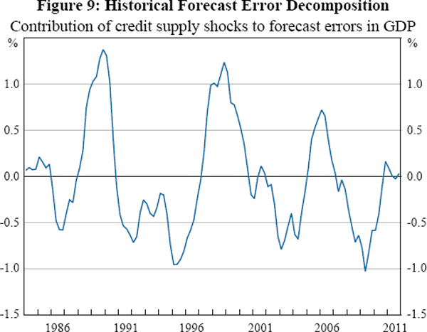
While credit supply stopped having a contractionary effect on GDP from mid 2010, this was not the case for business credit; credit supply shocks subtracted around 2½ per cent from business credit in mid 2010 and they were still having a contractionary effect as of December 2011.

While credit supply shocks had a sizeable effect on GDP during the global financial crisis, this event appears to have been shorter and sharper than that experienced in the early 1990s. The early 1990s episode saw a damaging credit cycle in Australia, associated with a deep and lengthy recession. Deregulation of the financial system through the 1980s had resulted in a substantial easing of lending standards, particularly to business borrowers. The result was a sharp rise in corporate gearing and prices of commercial property (which had been an important source of collateral). When this all unwound it produced widespread corporate failures and large losses for financial institutions (Kent and D'Arcy 2000; Macfarlane 2006). Consistent with the severity of this episode, the cumulative effect of negative credit supply shocks on GDP in our model is larger during the early 1990s than in the recent global financial crisis period.

5.3 Response to a Monetary Policy Shock

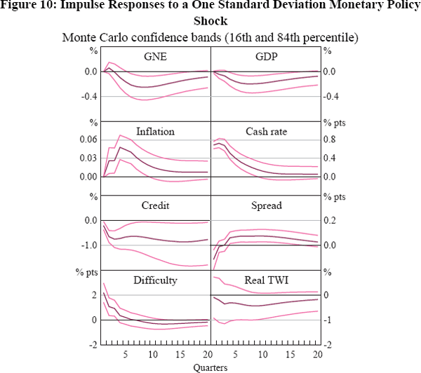
Figure 10 presents impulse responses to a one standard deviation monetary policy shock – that is, an unanticipated tightening in monetary policy. The results are consistent with a credit channel of monetary policy transmission. A monetary policy shock results in an immediate increase in the difficulty of obtaining finance and a gradual increase in credit spreads. Australian GDP falls by 0.2 per cent relative to its baseline 18 months after the shock. Business credit also declines following a monetary policy shock, and the decline is more persistent than it is for GDP. As with many other macroeconomic VAR models, our results present a ‘price puzzle’ – a rise in inflation following a contraction in monetary policy – although the magnitude of this effect is small (under 5 basis points).^[25] The direction of the exchange rate response is also consistent with a commonly found exchange rate puzzle, although it is statistically insignificant.

5.4 Net Worth and ‘Financial Accelerator’ Effects

In assessing the robustness of the model, we consider whether any important variables may have been omitted from the system of equations (other robustness checks are considered in the next section). Credit shocks can be misspecified if lenders change the availability of credit in response to variables that are not included in the system. In particular, the financial position of borrowers is likely to be taken into consideration by lenders when determining the price and non-price conditions of providing finance. This is a key component of the financial accelerator mechanism. Given this, we add a measure of net worth to our model that was considered in Lowe and Rohling (1993): the market capitalisation of listed equities on the ASX expressed as a ratio to business credit.^[26]

The identification of the model with net worth included is very similar to our baseline model, with a few small changes:

• The cash rate is assumed to respond contemporaneously to net worth since stock price data are available in a timely manner and developments in equity markets can be a leading indicator of future economic activity.
• Net worth is assumed to respond contemporaneously to GNE, GDP, inflation, the cash rate and the exchange rate.
• To allow for these new assumptions and ensure identification, we impose a zero restriction that was not imposed in the baseline model. Specifically, we assume that inflation responds to GNE and GDP only with a lag.

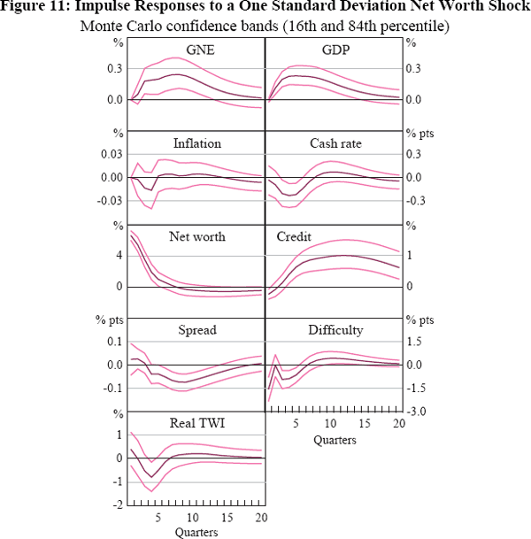
The inclusion of net worth in the model does not change the key results. In particular, a credit supply shock has broadly the same effects, resulting in a significant decline in GDP. Furthermore, consistent with the linkages described in financial accelerator models, we find that a positive shock to net worth results in a decline in the difficulty of obtaining finance, a decline in spreads and a rise in GDP and business credit (Figure 11).

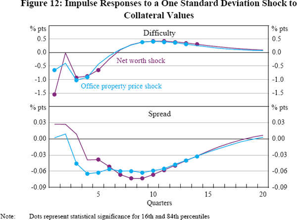
For many businesses, a key asset used as collateral against borrowing is commercial property. As discussed above, booms and busts in commercial property prices have often been a key feature of previous credit cycles in Australia (see Kent and D'Arcy (2000)). Accordingly, we also consider changes in office property prices as an alternative proxy for collateral values. The results are similar to the net worth model, with a positive shock to office property prices resulting in a fall in both the difficulty of obtaining finance and lending spreads (Figure 12). Other responses in the model, including the impact of a credit supply shock on GDP, are largely unchanged from our baseline model.

Footnotes

Ten thousand draws are taken and confidence intervals are generated using 16th and 84th percentiles (as proposed by Sims and Zha (1999) and as per the recommended settings in RATS Monte Carlo procedures). The main results remain significant when confidence intervals are generated using the 2.5 per cent and 97.5 per cent quantiles. Complete results from our baseline model are available on request. [23]

Note that these effects do not take account of the credit market's role in propagating shocks from other sources, but only reflect shocks identified as originating from the credit market itself. [24]

The price puzzle becomes statistically insignificant if a measure of inflation expectations is added to the model. [25]

A book value measure of net worth is likely to correspond more closely with the covenants contained in credit market contracts. However, book value data are not available for the full sample period, or at quarterly frequency. [26]