RDP 2013-08: International Business Cycles with Complete Markets 4. The Results
June 2013 – ISSN 1320-7229 (Print), ISSN 1448-5109 (Online)
- Download the Paper 736KB
4.1 Positive Cross-country Co-movement of Output, Investment and Hours
In this section we show that a model with complete markets driven by TFP shocks can account for the observed pattern of international co-movement of consumption, investment and hours worked. In fact, our model's predictive performance is remarkably similar to that of the model with incomplete markets proposed by Kehoe and Perri (2002).
We start by reviewing the puzzles. The first column of Table 2 displays cross-country correlations in aggregate quantities based on US data and that for the aggregate of 15 European countries. In column 2 we show the averages from 190 pairwise correlations among 20 industrialised countries reported by Ambler, Cardia and Zimmermann (2004). The last column reports predictions of the model with standard Cobb-Douglas preferences (no habits). This model fails along two dimensions. First, it predicts negative cross-country correlations in investment and employment while they are positive in the data. Second, in the data, international correlations of output and consumption are positive and fairly high, with the former exceeding the latter. This standard model predicts almost perfectly correlated consumptions and virtually uncorrelated outputs.
| Data | Model economy with: | |||||
|---|---|---|---|---|---|---|
| Europe –US | Average from ACZ | GHH preferences | Cobb-Douglas preferences | |||
| Habits | No habits | Habits | No habits | |||
| Output | 0.56 | 0.28 (0.03) | 0.25 | 0.21 | −0.05 | 0.01 |
| Consumption | 0.46 | 0.15 (0.03) | 0.56 | 0.48 | 0.92 | 0.90 |
| Investment | 0.43 | 0.22 (0.04) | 0.39 | −0.42 | 0.17 | −0.21 |
| Employment | 0.31 | 0.22 (0.03) | 0.23 | 0.21 | −0.75 | −0.49 |
| Solow residual | 0.36 | 0.21 (0.02) | 0.25 | 0.25 | 0.25 | 0.25 |
| Notes: The cross-country correlations in column 1 are calculated from US data and data aggregated over 15 European countries. The sample consists of time series covering the period of 1970:Q1–2008:Q2. The statistics in column 2 are taken from Table 1 in Ambler et al (2004) (ACZ), who consider all 190 pairwise cross-country correlations among 20 industrialised countries. Column 2 reports averages of these cross-country correlations and the standard deviations of the average correlations (in parenthesis) for the sample covering 1973:Q1–2000:Q4. Our benchmark model's predictions are reported in the column ‘GHH preferences/habits’. The model's statistics are computed from a single simulation of 100,000 periods. All the statistics are based on logged (except for net exports) and HP-filtered data with a smoothing parameter of 1,600. | ||||||
Our benchmark model, which incorporates GHH preferences and habits, resolves what Baxter (1995) calls the ‘international co-movement puzzle’. It matches the data by predicting positive cross-country correlations of investment and hours worked. The benchmark model moves in the right direction in accounting for the ‘quantity anomaly’ of BKK. It predicts a realistic level of international correlation of output (0.25 vs. 0.28 in the data). Relative to the model with Cobb-Douglas preferences, ours predicts a lower cross-country correlation of consumption (0.56 vs. 0.15 in the data). However, it fails to reverse the order of consumption and output correlations.
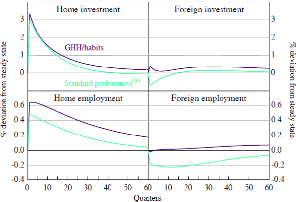
Figure 1 provides some additional insights. Following a positive productivity shock at home, foreign investment falls under Cobb-Douglas preferences while it rises in our benchmark model (GHH preferences with habits). What Backus et al (1995, p 340) call the tendency to ‘make hay where the sun shines’ does not apply to investment behaviour in our model. As Figure 1 suggests, the benchmark model predicts positive co-movement of investment even if the productivity innovations are uncorrelated.

Note: (a) Cobb-Douglas with no habits
In the aftermath of a positive shock at home, foreign employment falls under both specifications of preferences. The positive co-movement of hours worked reported in Table 2 for our benchmark model is observed because the productivity innovations in the two economies are contemporaneously correlated. In the case of both standard Cobb-Douglas preferences without habits and our benchmark model featuring GHH preferences with habits, the wealth effect tends to decrease foreign hours worked while home employment rises. However, the magnitude of the wealth effect is far smaller under GHH preferences with habits. This explains the reversal of the sign on the cross-country employment correlation.
4.2 Elements of the Model
In this section we discuss the role played by each of the three features of the model. We also describe how all three ingredients are necessary for our result.
4.2.1 Capital adjustment costs
Costly capital adjustment has two roles to play. First, it dampens the unrealistically high volatility of investment relative to output.[5] Second, it complements habits in restricting the immediate response of domestic absorption, c(st) + i(st), to a productivity shock. In our model, the latter feature is necessary to account for the positive cross-country correlation of investment.
4.2.2 GHH preferences
Under GHH preferences, the marginal rate of substitution between consumption and leisure is independent of consumption. The first order condition for labour, Equation (12), shows that GHH preferences eliminate the wealth effect on labour supply as well as eliminating intertemporal substitution of leisure
The absence of wealth effects on labour supply is responsible for the positive international correlation in hours worked. To see this, consider the log-linearised version of Equation (12)
where  and
and  denote the percentage deviation of the corresponding variable from its steady state.
Since k(st−1) is predetermined
at t, positively correlated innovations to productivity translate
into positive co-movement of hours worked. The latter translates into a positive
cross-correlation in output levels.
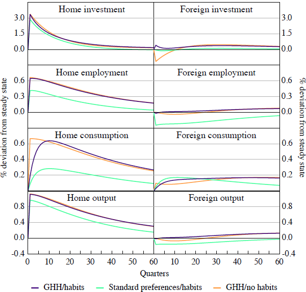
Figure 2 and Table 2 show that a model featuring GHH preferences but no habits fails to account for the co-movement puzzle. It cannot get the positive investment co-movement right. The tendency to ‘make hay where the sun shines’ is still present. Investment rapidly moves to the most productive location.

Under GHH preferences with no habits, after a positive productivity shock at home, investment at home rises while foreign investment falls. The fact that innovations to TFP are contemporaneously correlated does little to change this pattern. In fact, Table 2 shows that investment is more negatively correlated under GHH preferences with no habits (column 4) than under Cobb-Douglas preferences (column 6). A similar result is reported in Raffo (2008) who considered a two-country, two-good economy with a GHH preference structure.
4.2.3 Internal habit formation
When we introduce linear internal habits in consumption, the marginal utility of consumption consists of two terms. The first term measures an increase in utility from consuming an extra unit. The second term captures expected discounted future disutility from today's increase in consumption.
Habit-forming households strive to smooth not only consumption but also changes in consumption. In the periods following the shock, they increase consumption gradually and allow their habits to adjust. Therefore, on impact, an increase in domestic output compels domestic agents to drastically increase their savings. Since rapid changes in the capital stock at home are costly, the domestic economy responds by increasing net exports. At the same time, foreign agents want to raise their consumption due to the wealth effect. However, habit formation punishes rapid changes in consumption. As a result, world output rises with minor changes to world consumption. An increase in world saving raises investment abroad provided that the adjustment cost at home exceeds the opportunity cost of not investing in the most productive location (i.e. the home country).
The introduction of consumption habits in the Cobb-Douglas class of preferences improves the cross-country correlation of investment. This improvement comes at a cost. The model predicts almost perfectly negatively correlated hours worked. One reason for this failure is the mechanism through which the wealth effect operates on labour supply.
4.3 International Transmission of Productivity Shocks: Combining the Elements
When consumption habits are introduced in the GHH class of preferences, the marginal utility of consumption becomes forward-looking
In contrast, the marginal disutility from work does not become forward-looking:
The static optimality condition that controls labour supply now reads as
where  .
The term Δ(st) measures the difference between the
overall and immediate increase in utility from an extra unit of consumption.
Since Δ(st) depends on current consumption, its presence
in Equation (13) re-introduces the wealth effect on labour supply. Its magnitude
depends on the intensity of habits, b. Therefore, the wealth effect
can be made arbitrarily small by choosing b close to zero. This feature
also appears in Jaimovich and Rebelo (2009) who introduce time non-separable
preferences consistent with arbitrarily small wealth effects.
The log-linearised version of Equation (13) is given by
As we have already noted, k(st−1) is predetermined at t.
The Δ(st) are equated across countries due to perfect
risk-sharing. International co-movement of hours will depend on the covariance
of  and
and  (that is, between the log-linearised productivity shock and the log-linearised Δ(st)).
Figure 1 shows that under GHH preferences with internal habits, foreign employment
falls slightly when home country productivity rises. Leisure is thus a normal
good and the terms
  and
and  co-move negatively.
Table 2 shows that the cross-country correlation of employment is slightly
higher in our benchmark than under GHH preferences with no internal
habits (0.23 vs. 0.21). Hence, the wealth effect on labour supply is
fairly small for our benchmark value of habit intensity.
The positive co-movement of hours reinforces the mechanism behind the positive co-movement of investment. Since foreign hours do not fall substantially in response to an increase in home productivity, there is a much greater response of global output. This creates additional savings that are channelled into foreign as well as home investment, enhancing the investment co-movement.
4.4 Additional Results
In this section we comment on our model's ability to match the features of within-country business cycles. We discuss how variation in the persistence of shocks and their degree of spillover affects our model's ability to account for international co-movements in the quantity aggregates. This is followed by some sensitivity experiments in Section 4.5.
4.4.1 Within-country business cycles
The within-country business cycle properties of the model featuring GHH preferences with habits are slightly better than those of the model with standard preferences (see Table 3). In particular, the volatilities of consumption, employment and output fit the data more closely. As expected, internal habits induce higher persistence in consumption, which results in a better fit to the data. These improvements are balanced by some deterioration, notably for the within-country correlations with output.
| Data | Model economy with: | ||||
|---|---|---|---|---|---|
| US | GHH preferences | Cobb-Douglas preferences | |||
| Habits | No habits | Habits | No habits | ||
| Panel A: Volatilities – standard deviation (per cent) | |||||
| Output | 1.51 | 1.48 | 1.49 | 1.26 | 1.31 |
| Net exports/output | 0.74 | 0.18 | 0.40 | 0.32 | 0.25 |
| Standard deviations relative to output | |||||
| Consumption | 0.81 | 0.44 | 0.62 | 0.28 | 0.36 |
| Investment | 2.88 | 2.88 | 2.88 | 2.88 | 2.88 |
| Employment | 0.84 | 0.58 | 0.59 | 0.46 | 0.48 |
| Solow residual | 0.58 | 0.62 | 0.62 | 0.73 | 0.70 |
| Panel B: Correlations with output | |||||
| Consumption | 0.86 | 0.75 | 0.99 | 0.67 | 0.84 |
| Investment | 0.94 | 0.95 | 0.92 | 0.97 | 0.97 |
| Employment | 0.88 | 0.99 | 0.99 | 0.92 | 0.96 |
| Net exports/output | −0.35 | 0.56 | −0.42 | 0.69 | 0.40 |
| Solow residual | 0.87 | 0.99 | 0.99 | 0.98 | 0.99 |
| Panel C: Autocorrelations | |||||
| Output | 0.87 | 0.74 | 0.73 | 0.73 | 0.73 |
| Consumption | 0.88 | 0.93 | 0.73 | 0.93 | 0.74 |
| Investment | 0.90 | 0.67 | 0.70 | 0.68 | 0.71 |
| Employment | 0.92 | 0.74 | 0.73 | 0.74 | 0.73 |
| Net exports/output | 0.86 | 0.54 | 0.74 | 0.76 | 0.94 |
| Solow residual | 0.75 | 0.71 | 0.71 | 0.71 | 0.71 |
| Notes: Domestic statistics in the Data column correspond to the US time series sample 1970:Q1–2008:Q2. The Solow residuals are constructed using GDP and employment data as described in BKK. The model's statistics are computed from a single simulation of 100,000 periods. All the statistics are based on logged (except for the net exports) and HP-filtered data with a smoothing parameter of 1,600. | |||||
A model with a time separable version of GHH preferences delivers a countercyclical net export to output ratio, matching an important feature of the data. Hence, we replicate the main result of Raffo (2008) in a model without relative price movements or trade in intermediate goods. As in Raffo, this result comes at a cost. The model fails to account for positive international co-movement of investment. Incorporating consumption habits changes the sign of both the investment co-movement and the labour co-movement by reducing the response of domestic absorption to a productivity shock. Similarly to Kehoe and Perri's (2002) model with limited commitment, our benchmark model predicts a positive cross-country investment correlation while it fails to generate countercyclical net exports.
4.4.2 Can we dispense with near-unit-root shocks without spillovers?
Having incomplete asset markets has helped to improve the empirical fit of international RBC models. Yet a known weakness of incomplete markets models is the sensitivity of their predictions to the parameterisation of the driving process. Baxter and Crucini (1995) illustrate this point in the case where international trade is restricted to non-contingent bonds. They show that the abilities of a complete markets economy and a bond economy to match the data are virtually the same unless TFP shocks follow a near-unit-root process without cross-country spillovers. Kehoe and Perri (2002) report a related result in an environment with endogenously incomplete markets. Their model predicts a negative cross-correlation of employment if the shocks follow the stationary process with mild spillovers used by Backus et al (1992).
There seems to be little consensus in the literature regarding the magnitude of spillover or persistence parameters of the TFP process. As Baxter and Farr (2005, p 340) note ‘[i]t has proved impossible to estimate the parameters of [the productivity process] with much precision’. This raises the question of whether our model allows us to dispense with near-unit-root shocks without spillovers.
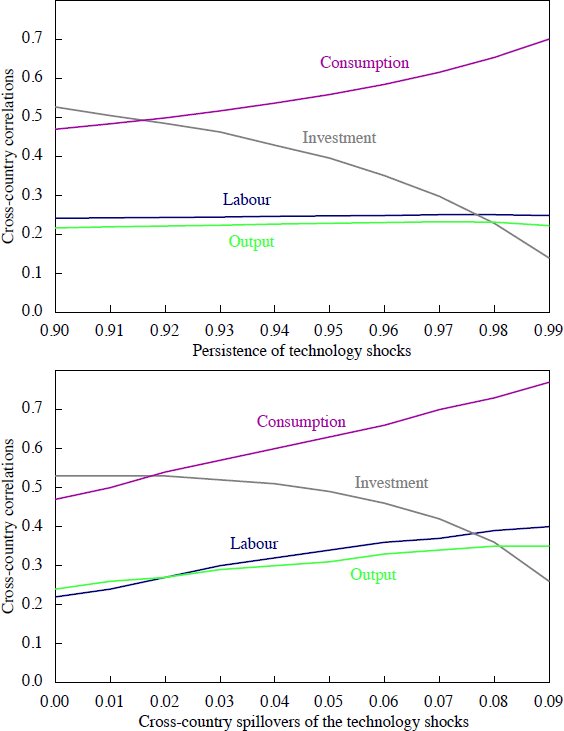
Figure 3 and Table 4 show how variation in spillover and persistence parameters affects our model's ability to account for international co-movement in quantity aggregates. The results can be summarised as follows. First, the implications of our model for the quantity anomaly are robust. Cross-country correlations of investment and hours remain positive for commonly used parameter values. Second, the two most sensitive statistics are international correlations of consumption and investment. Third, a higher degree of spillovers leads to a higher cross-correlation of consumption and a lower cross-correlation of investment. Finally, a lower degree of persistence leads to a lower cross-country correlation of consumption and a higher cross-correlation of investment. The intuition for the latter is as follows. The less persistent the shocks are, the less inclined habit-forming individuals are to change their consumption profiles. In the more-productive country this implies higher investment, saving and, therefore, net exports after a positive TFP shock. This increase in net exports, coupled with foreign individuals' reluctance to change consumption, leads to higher investment in the less-productive economy as well. The sensitivity of crosscountry correlations of investment and consumption to the persistence parameter highlights the central role of internal habits in getting the investment co-movement right.

| Data | Benchmark model | Variations | |||||
|---|---|---|---|---|---|---|---|
| BKK productivity process | Persistence of shocks | Frisch elasticity | |||||
| Low (ρ = 0.9) | High (ρ = 0.98) | Low (εf = 1) | High (εf = 1.8) | ||||
| Panel A: Volatilities – standard deviation (per cent) | |||||||
| Output | 1.51 | 1.48 | 1.83 | 1.45 | 1.49 | 1.36 | 1.57 |
| Net exports/output | 0.74 | 0.18 | 0.20 | 0.24 | 0.12 | 0.20 | 0.17 |
| Standard deviations relative to output | |||||||
| Consumption | 0.81 | 0.44 | 0.54 | 0.39 | 0.50 | 0.41 | 0.46 |
| Investment | 2.88 | 2.88 | 2.88 | 2.88 | 2.88 | 2.88 | 2.88 |
| Employment | 0.84 | 0.58 | 0.61 | 0.58 | 0.58 | 0.49 | 0.64 |
| Panel B: Correlations with output | |||||||
| Consumption | 0.86 | 0.75 | 0.75 | 0.74 | 0.76 | 0.75 | 0.76 |
| Investment | 0.94 | 0.95 | 0.91 | 0.95 | 0.94 | 0.95 | 0.95 |
| Employment | 0.88 | 0.99 | 0.99 | 0.99 | 0.99 | 0.99 | 0.99 |
| Net exports/output | −0.35 | 0.56 | 0.36 | 0.59 | 0.47 | 0.56 | 0.56 |
| Panel C: Autocorrelations | |||||||
| Output | 0.87 | 0.74 | 0.72 | 0.71 | 0.75 | 0.73 | 0.74 |
| Consumption | 0.88 | 0.93 | 0.93 | 0.93 | 0.93 | 0.93 | 0.93 |
| Investment | 0.90 | 0.67 | 0.63 | 0.65 | 0.67 | 0.67 | 0.67 |
| Employment | 0.92 | 0.74 | 0.72 | 0.72 | 0.76 | 0.74 | 0.75 |
| Net exports/output | 0.86 | 0.54 | 0.81 | 0.56 | 0.53 | 0.60 | 0.49 |
| Panel D: Cross-country correlations | |||||||
| Output | 0.56 | 0.25 | 0.35 | 0.24 | 0.25 | 0.25 | 0.25 |
| Consumption | 0.46 | 0.56 | 0.79 | 0.47 | 0.65 | 0.63 | 0.52 |
| Investment | 0.43 | 0.39 | 0.14 | 0.53 | 0.23 | 0.43 | 0.36 |
| Employment | 0.31 | 0.23 | 0.40 | 0.22 | 0.23 | 0.23 | 0.23 |
| Notes: Domestic statistics in the Data column correspond to the US time series sample 1970:Q1–2008:Q2. The cross-country correlations in this column are calculated from US data and data aggregated over 15 European countries. The model's statistics are computed from a single simulation of 100,000 periods. All the statistics are based on logged (except for the net exports) and HP-filtered data with a smoothing parameter of 1,600. | |||||||
4.5 Sensitivity Experiments
As discussed in Section 3, the benchmark values for two preference parameters are taken from the literature. Here we report how changes in the parameterisation of habit intensity b and the Frisch elasticity of labour supply 1/η affect our model's predictions for international co-movements.
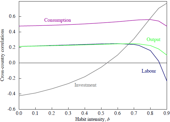
Habit intensity Figure 4 shows the extent to which cross-correlations of consumption, investment, output and employment depend on the strength of habit formation. There are three key results. First, the cross-country investment correlation is increasing as habit formation intensifies. The larger b is, the more the consumer is interested in smoothing the change rather than the level of consumption. Hence, for small b the model is similar to the model with time separable preferences. Second, the cross-country correlation of hours worked remains positive as long as b < 0.86. As b increases further, the positive correlation of TFP innovations fails to compensate for the stronger wealth effect on labour supply. Third, the international correlations of consumption and output levels remain positive for the entire range of b. The gap between the two moments shows almost no dependence on habit intensity.

Labour supply elasticity Our results show little sensitivity to variation in the Frisch elasticity of labour supply. In our experiments, we considered the range between 1 and 1.8, which corresponds to the estimates by Chang and Kim (2006) and Fiorito and Zanella (2008). Table 4 illustrates the differences between our benchmark case (1/η = 1.43), the ‘low elasticity’ case (1/η = 1), and the ‘high elasticity’ case (1/η = 1.8). Decreasing the labour supply elasticity moderates the volatility of output and hours worked. The rest of the business cycle statistics remain virtually unaffected.
Footnote
Most two-country business cycle models rely on adjustment costs to curb investment volatility. This applies to complete market models (Raffo 2008), as well as models with restricted markets (Baxter and Crucini 1995). A notable exception is Kehoe and Perri (2002), where an endogneously incomplete market framework delivers plausible investment volatility. [5]


