RDP 2014-12: A State-space Approach to Australian GDP Measurement Appendix B: Levels or Differences?
October 2014 – ISSN 1320-7229 (Print), ISSN 1448-5109 (Online)
- Download the Paper 904KB
Our baseline models relate the growth rate of GDP to its expenditure, income and production measures. We focus on growth rates because it is the growth rate of GDP (and its implications for the output gap), rather than its level in dollars, that is of day-to-day interest to policymakers. However, even if we are most interested in GDP growth, the level of GDP may still contain useful information, particularly as the three ABS measures should be cointegrated. To examine whether accounting for the level of GDP affects our results, we modified our models to allow for cointegration between GDP and the expenditure, income and production measures. To do this, we augment our basic measurement equation to include an error correction term:
for j ∈ {E,I,P} where  and yt
are the log-levels of a measure of GDP and the unobserved ‘true’
measure of GDP. The parameter ηj tells us how quickly
the levels of a measure of GDP and its ‘true’ value converge.
The state-space form and estimation procedure of this model is similar to our baseline models, although we adjust the Kalman filter to account for the fact that the level of GDP is non-stationary. We do this using the methods of Koopman and Durbin (2003).
Table B1 shows the results for Model 2 estimated in error correction form (ECM). In most cases, the parameter estimates are similar to those in the equivalent model estimated in growth rates. However, the variances of some of the shocks are smaller in the ECM model. And the negative relationship between innovations to GDP and the measurement errors ceases to be statistically significant. The error correction term in the GDP(I) equation is larger than those in the equations for the other two observed measures of GDP. That is, deviations of the level of GDP(I) from the true GDP appear to close more rapidly than those of other measures. Most of these deviations, however, are likely to have occurred in the early years of the sample. The ABS reconciliation process ensures that for all years since 1994, and before the latest financial year, the sums of GDP(E), GDP(I) and GDP(P) over a financial year are equal.[22] Hence, it is unlikely that any of these series could deviate from true GDP for a substantial period of time.
| Parameter | Distribution | Prior | Posterior | |||||
|---|---|---|---|---|---|---|---|---|
| Mean | Std dev | Mode | Median | 5% | 95% | |||
| GDP equation | ||||||||
| μ | Normal | 0.80 | 10 | 0.73 | 0.74 | 0.56 | 0.91 | |
| ρ | Beta | 0.50 | 0.2 | 0.55 | 0.54 | 0.36 | 0.73 | |
| Exogenous processes | ||||||||
 |
Inv Gamma | 2 | 4 | 0.25 | 0.28 | 0.17 | 0.39 | |
| σGE | Normal | 0 | 10 | −0.10 | −0.09 | −0.22 | 0.03 | |
| σGI | Normal | 0 | 10 | −0.11 | −0.07 | −0.28 | 0.12 | |
| σGP | Normal | 0 | 10 | −0.15 | −0.14 | −0.26 | −0.03 | |
 |
Inv Gamma | 2 | 4 | 0.57 | 0.58 | 0.39 | 0.81 | |
| σEI | Normal | 0 | 10 | 0.18 | 0.19 | 0.02 | 0.38 | |
| σEP | Normal | 0 | 10 | 0.24 | 0.24 | 0.08 | 0.42 | |
 |
Inv Gamma | 2 | 4 | 0.46 | 0.56 | 0.36 | 0.80 | |
| σIP | Normal | 0 | 10 | 0.15 | 0.15 | −0.03 | −0.34 | |
 |
Inv Gamma | 2 | 4 | 0.48 | 0.50 | 0.34 | 0.69 | |
| Error correction terms | ||||||||
| ηE | Beta | 0.5 | 0.2 | 0.37 | 0.43 | 0.27 | 0.70 | |
| ηI | Beta | 0.5 | 0.2 | 0.87 | 0.70 | 0.38 | 0.92 | |
| ηP | Beta | 0.5 | 0.2 | 0.23 | 0.24 | 0.15 | 0.33 | |
| Marginal data density 249.22 | ||||||||
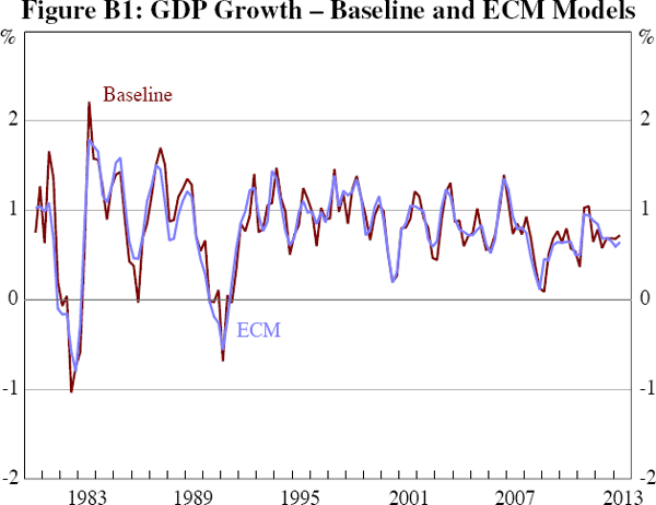
Figure B1 compares the GDP series from the ECM model with the equivalent series derived from our baseline model. Compared with the baseline model, the ECM model smooths some of the peaks and troughs in GDP growth. This is particularly noticeable in the 1980s and early 1990s. The 1986 growth slowdown is hardly noticeable in the ECM series while the early 1980s and 1990s recessions are shallower but more prolonged.

Footnote
The ABS reconcile the measures of GDP using annual supply-use tables. Due to lags in compiling the tables, the measures of GDP are not equal for the most recent financial year (or two years in the case of the June quarter). [22]
