RDP 2015-03: The Value of Payment Instruments: Estimating Willingness to Pay and Consumer Surplus Appendix B: Methodology – Estimation of Willingness to Pay

The methodology used to estimate willingness to pay follows the model developed by Hanemann et al (1991) for double-bounded DCE data.

For all N number of consumers, the ith consumer's willingness to pay (our variable of interest) to use a card instead of cash is specified as a continuous latent random variable represented by:

Here α is the mean willingness to pay (when all independent variables are zero), x_i is the vector of independent variables, β is the vector of coefficients and ε_i is the normally distributed random error term with σ² variance.

To obtain the estimates for the above parameters, the latent variable is mapped to the discrete data we observe, which is denoted by y_{i, pl, pu} and takes the values:

where y_{i, pl , pu} is the indicator flag taking the value 1 if consumer i's willingness to pay lies between the lower bound price p_l and upper bound price p_u, or taking the value zero otherwise. p_l is an element of the set L of lower bound prices (in basis points) of {−∞,10,50,75,100,200,300,400}. A corresponding p_u, which is an element of the set U of upper bound prices {10,50,75,100,200,300,400,∞}, exists for each p_l. The eight ranges of willingness to pay in basis points are:

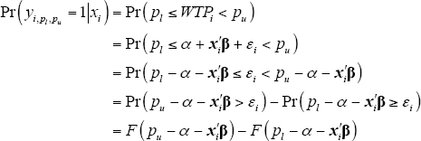
The probability of respondent i having a willingness to pay within the range bound by p_l and p_u is given by:

where F() is the (non-standard) normal cumulative distribution function of ε_i.

The log-likelihood function for the full sample is given by:

where p_l ∈L, p_u ∈U refers to the eight pairs of price points referred to above (as opposed to every combination of the price bounds).

The log-likelihood function is maximised using a Newton-Raphson numerical optimisation procedure in Stata.

B.1 Calculation of the truncated mean

The mean of the normal distribution above the truncation point is as derived in Greene (2012):

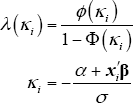
where , following the specification above. The inverse Mills ratio λ(κ) for a distribution that is truncated at zero for values below zero is:

where ϕ is the standard normal density function and Φ is the standard normal cumulative distribution function.

The mean of the distribution above the truncation point is then multiplied by the proportion of the distribution above the truncation point to arrive at the mean of the whole distribution.