RDP 2015-14: Okun's Law and Potential Output 6. Specification Issues
December 2015 – ISSN 1448-5109 (Online)
- Download the Paper 987KB
6.1 Asymmetry
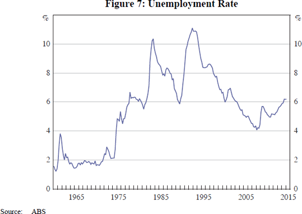
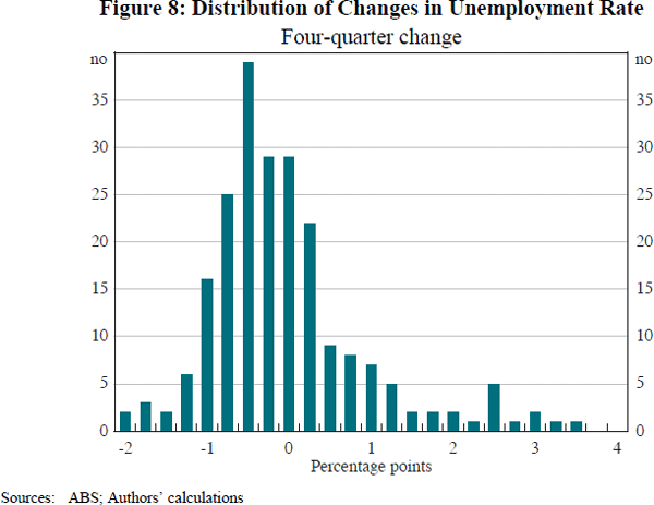
A striking feature of the unemployment rate is that the distribution of changes is asymmetric. As shown in Figure 7, the unemployment rate tends to go up quickly, and down slowly. (The gradual increase over 2013 and 2014 is an exception.) Figure 8 shows the distribution of four-quarter changes. The most common outcome is a small decline. There are several very large increases of over 3 percentage points, but no decreases of more than 2 percentage points. This skewness is also evident in changes in other frequencies and in other countries.


Table 2 shows a standard measure of asymmetry, the skewness statistic. We exclude the first few years from the calculations, to allow the diffuse priors about our state variables to tighten. For this sample, the skewness of quarterly changes in the unemployment rate is 1.60. For a sample of the same size, a normally distributed variable would exhibit skewness this large less than 0.01 per cent of the time.[11]
| Skewness statistic | p-value (%); H0 = 0 | |
|---|---|---|
| Unemployment rate, quarterly change | 1.60 | < 0.01 |
| Output gap, two-quarter change (constant coefficients model) |
−0.32 | 3.29 |
| Output gap, two-quarter change (time-varying coefficients model) |
−0.84 | < 0.01 |
| Okun's law model with time-varying coefficients | ||
| Predicted change in unemployment rate | 1.53 | < 0.01 |
| Measurement equation residuals | 0.94 | < 0.01 |
The asymmetry of changes in the unemployment rate is largely, though not entirely, explained by our model. Changes in the output gap are also skewed, especially when potential output growth varies over time (skewness = −0.8, p < 0.01 per cent). Moreover, the interaction of changes in the output gap with the other regressors results in predicted values of our model that are similarly skewed as changes in the unemployment rate. There remains some unexplained skewness in the residuals (skewness = 0.9, p < 0.01 per cent), but it is much smaller than the skewness in the fitted values (skewness = 1.5, p < 0.01 per cent). That is, we explain most, though not all, of the skewness in the data.
The unemployment rate rises quickly in recessions and falls slowly in expansions. Although our model explains most of this asymmetry, an alternative explanation is that the response of unemployment to changes in the output gap is nonlinear. To assess this, we interact the change in the output gap with a ‘boom’ dummy variable that equals one when the output gap is increasing and zero otherwise. This variable is not significantly different to zero (p = 39 per cent). Ball et al (2013) conduct a similar test on US data and find similar results.
We consider other specifications. Some of these variations were marginally significant but difficult to interpret (for example, implying discontinuous relationships). Others were insignificant. Having experimented with a range of functional forms, we have not found clear evidence that the relationship between output growth and changes in unemployment is nonlinear.
6.2 Changes in the NAIRU
Okun's law equations like Equations (3) and (4) are often estimated with the dependent variable being the change in the unemployment gap (the deviation of the unemployment rate from the NAIRU) rather than the change in the unemployment rate. From a forecasting perspective, these variables are typically the same, as the NAIRU is conventionally modelled as a random walk. But for explaining history, we find that this specification fits the data poorly. We update the domestic demand deflator version of the NAIRU estimated by Ballantyne, De Voss and Jacobs (2014) and include the contemporaneous quarterly change in the one-sided NAIRU in Equation (4). The coefficient is incorrectly signed and is not significantly different from zero (p = 6 per cent). In this specification, the expected growth rate of potential output is about half a percentage point higher in the 1970s and about half a percentage point lower in the 2000s than the estimates shown in Figure 2, though the 2015:Q1 estimate is unchanged at 2.9 per cent. The hypothesis that the dependent variable is the change in the gap, which implies constraining the coefficient on the change in the NAIRU to equal one, is very strongly rejected (p < 0.1 per cent). The hypothesis that the coefficient equals 1 − αt (allowing for interaction with the lagged dependent variable) also has p < 0.1 per cent. Ballantyne et al's weighted median version of the NAIRU provided an even poorer fit to the data.
6.3 Levels of Potential Output and Equilibrium Unemployment
In contrast to most previous research on potential output and Okun's law, we do not present estimates of levels of potential output, the output gap or the equilibrium rate of unemployment. We have not been able to construct estimates that are useful for explaining unemployment. For example, the lagged level of the unemployment rate and a constant (allowing for reversion to the mean or to the NAIRU) are jointly insignificant with a p-value of 17 per cent when included in a least squares version of our equation. (We constrain time-varying coefficients to equal their Kalman filter estimates, so as to avoid collinearity between the constant and potential output growth.) Similarly, the lagged output gap, constructed as the deviation of log GDP from its one-sided HP trend, has a coefficient that is insignificantly different from zero (p = 25 per cent). More sophisticated specifications, including cyclically adjusted estimates and one-sided estimates of the NAIRU, do not do much better. This is not primarily because our time-varying coefficients soak up the effect of the levels variables. When the lagged deviations of log GDP and the unemployment rate from their one-sided HP trends are included in our constant coefficients specification (as shown in Table 1) they are individually and jointly insignificant (p = 43 per cent).
To be clear, we are not saying that the relationship between unemployment and output does not hold in levels. Rather, variables in levels do not seem to provide information about changes in unemployment beyond the information provided by variables in changes.
The insignificance of level terms may seem surprising given the stationarity (absence of trend) of the unemployment rate. In the past, when the unemployment rate was far from its average, it returned toward normal. Our estimates suggest that this mean reversion arises through output growing faster or slower than normal. Once one allows for that, extra reversion to the mean is unimportant.
Exceptions to our findings above are specifications that include two-sided trends (whether HP, kinked linear or Kalman) of both output and the unemployment rate. Like Ball et al (2013) we find these terms to be highly statistically significant. But this correlation seems to reflect reverse causation. In particular, disturbances to the unemployment rate result, by construction, in positively correlated changes in the lagged HP trend.
To illustrate, we construct artificial data resembling our unemployment rate and
Ball et al's (2013) NAIRU, in which the null hypothesis,
that the NAIRU has no effect on the unemployment rate, is true by construction.
Specifically, we simulate 50,000 unemployment rate series, each of 219 observations,
taking the right-hand side variables and coefficients of the time-varying model
as given and random draws of disturbances from a normal distribution, where
 ~ N (0,0.2332). We then construct a HP trend of the cumulative
sum of each series using the same procedure as Ball et al
(2013) (with a smoothing coefficient λ = 1,600). Although the
artificial unemployment data are constructed independently of the artificial
NAIRU series, when included in our Okun's law model, the resulting lagged
level of the unemployment gap usually appears to be highly significant, with
an average t-statistic of −4.2. At a 5 per cent level of significance,
a t-test on the lagged deviation of the unemployment rate from its
HP trend incorrectly rejects the null hypothesis of a zero effect 99.8 per
cent of the
time.[12]
We conclude that the finding that the unemployment rate moves towards a two-sided
trend of itself is spurious. That is, Ball et al (2013)
overstate the evidence that Okun's law holds in levels. This conclusion
applies in essentially the same way to kinked linear trends and two-sided Kalman
trends. We should add that, in contrast, our other results strongly corroborate
Ball et al's findings relating to Okun's law in
changes.
Footnotes
All p-values in this section are generated by Monte Carlo. We take 100,000 draws of 202 observations of a normal random variable to create the distribution of skewness statistics. [11]
These results are not materially different if we draw disturbances from the empirical distribution of ε, vary the standard deviation of the residuals or use an alternative value of lambda. [12]