Research Discussion Paper – RDP 2016-11 Identifying Interbank Loans from Payments Data
1. Introduction
The average interest rate on unsecured overnight interbank loans – the cash rate – is the Reserve Bank of Australia's (RBA) operational target for monetary policy. Moreover, the market for these loans (known as the interbank overnight cash (IBOC) market) is the market most directly affected by the RBA's standing facilities, and the RBA has control over the supply of funds in this market.[1] So this market represents the first step in the transmission of monetary policy to the rest of the economy, meaning its smooth operation is critical for the financial and economic system. Consequently, it is important for the RBA to have detailed knowledge about this market.
While central banks have a wealth of information on interbank payments, there has historically been no in-built ability to distinguish the payments that constitute loans from other types of payments (other payments include those between banks' customers and foreign exchange transactions).[2] Moreover, other sources of information about these loans do not typically include the level of detail that would be available in a loan-level dataset. For example, the RBA's Interbank Overnight Cash Rate Survey (IBOC Survey) only provided the aggregate gross value of each survey participant's IBOC lending and borrowing during each trading session of the day, and the average interest rate at which these loans occurred.[3]
To garner detailed information on IBOC loans, algorithms have been developed to identify the interbank payments that constitute these loans. These algorithms are typically based on the seminal work of Furfine (1999), but have since been extended along several dimensions (see Demiralp, Preslopsky and Whitesell (2004) and Hendry and Kamhi (2007), for example). Given the mixed success of these algorithms (see Appendix A for details), we build on this literature to design a new algorithm for use in Australia (detailed in Section 3).
The main innovation of our algorithm is the ability to identify ‘rollovers’. A rollover occurs when, instead of repaying a loan from the previous day, the lender and borrower agree to a new IBOC loan. The lack of next-day repayment makes rollovers difficult to separately identify from longer-term loans. As a result, even though previous international research has discussed the possibility of rollovers (e.g. Furfine 1999; Armantier and Copeland 2015; Arciero et al 2016), existing algorithms do not attempt to identify them.
Identifying rollovers introduces complications beyond the lack of daily repayments. For example, borrowers could pay interest on a daily basis even though the principal of the loan is rolled over, or all interest could be paid when the loan ceases to be rolled over (with interest not necessarily included in the same payment as the principal). Interest may also be calculated in different ways (i.e. simple or compound). Our algorithm allows for all of these possibilities.
Perhaps the biggest innovation of our algorithm is the ability to identify rollovers for which only part of the principal is rolled over, or for which the principal is increased. In this case, daily payments only reflect the change in principal, and the dollar value of daily interest varies over the rollover period (with the changes in principal). For reasons that will be explained in Section 3, identifying this type of rollover requires an algorithm that is fundamentally different to a Furfine-type algorithm.
By comparing aggregates of the IBOC loans identified by our algorithm to IBOC Survey data, we conclude that our algorithm successfully identifies the majority of IBOC loans. Between 2005 and 2015, the daily correlations between the IBOC Survey data and the algorithm output are greater than 90 per cent (increasing to 96 per cent for the four major Australian banks). As is discussed in Section 4, such accuracy is uncommon in the existing literature, which may be partially due to the inability of existing algorithms to identify rollovers (the daily correlations in our sample drop below 40 per cent if rollovers are excluded). So the novel features of our algorithm may also be useful for identifying overnight interbank loans in other countries.
The loan-level dataset produced by our algorithm contains information on counterparties, loan values, interest rates, time of settlement, time of repayment, rollover length, and repayment structures. With the most detailed IBOC market dataset ever constructed now at our disposal, we explore several features of the market that were previously unobservable. The aim is to both improve our understanding of how the market functions, and help explain several of the changes that have occurred over the past decade, for example (see Section 5 for details):
- The halving of IBOC market activity between 2009 and 2015 mainly involved an 87 per cent fall in the value of rollovers (rollovers accounted for almost half of the market before the fall), with the value of non-rolled loans being little changed.
- While both rollovers and non-rolled loans appear to be used to satisfy banks' late-day funding needs, they are not perfect substitutes, with rollovers conducted earlier in the day (when banks may be less certain of their late-day funding requirements). Knowing the timing of loans is important for operational decisions made by the RBA (such as the timing of open market operations).
- Banks are currently conducting non-rolled lending during a briefer period (towards the end of the day) than has been the case historically. And, despite significant changes to the market resulting from the introduction of same-day settlement of direct entry obligations in November 2013, there is little evidence that these changes affected the timing of non-rolled IBOC loans.
- Simple interest was used to calculate the repayments of rollovers, even though daily interest typically remained outstanding for the life of the rollover.
The main advantage of this new loan-level database is the ability to conduct previously infeasible analyses of the IBOC market, such as forthcoming analysis of how the market changed during the global financial crisis.
2. The Australian Payments System and IBOC Market
This section is based on RBA Bulletin articles that analyse Australia's high-value payments system and IBOC market (Baker and Jacobs 2010; Gallagher, Gauntlett and Sunner 2010; Fraser and Gatty 2014), and information available on the RBA website (RBA 2009a, 2009b, 2012, 2015b, 2015c, 2016). Readers familiar with the Australian payments system and IBOC market may skip this section.
Australia's high-value payments system is the Reserve Bank Information and Transfer System (RITS). RITS is used by banks and other approved institutions to settle payment obligations on either a real-time gross settlement (RTGS) basis or periodically on a multilaterally netted basis. RITS is open on days when banks are generally open for business in Sydney or Melbourne.
RTGS transactions are entered into RITS either directly (known as ‘cash transfers’) or indirectly via external feeder systems (either the SWIFT Payment Delivery System or Austraclear). The Austraclear system provides settlement facilities for wholesale debt securities and money market transactions. The SWIFT system is predominantly comprised of payments between banks' customers and the Australian dollar leg of foreign exchange transactions.
Market liaison suggested that the majority of IBOC loans were executed using cash transfers, but that some participants preferred to use Austraclear. Due to the large number of SWIFT transactions (91 per cent of all RTGS transactions during 2009/10 – see Gallagher et al (2010)), and market liaison suggesting that this payment system was unlikely to be used to settle IBOC loans, our research only uses RTGS transactions entered either directly or via Austraclear.[4]
RITS transactions are settled using Exchange Settlement Accounts (ESAs). These are accounts ‘held at the Reserve Bank of Australia by financial institutions to settle financial obligations arising from the clearing of payments’ (RBA 2009b). ESAs are mandatory for all Australian-licensed banks and for other authorised deposit-taking institutions with RTGS transactions of at least 0.25 per cent of the total value of RTGS transactions. Financial institutions that do not meet these requirements may also be eligible for ESAs. For simplicity, this paper will refer to any financial institution with an ESA as a ‘bank’.
The IBOC market is used by banks to manage their liquidity. ESAs must remain in credit at all times; banks borrow in the IBOC market to ensure they satisfy this requirement (as the cost of overnight borrowing from the RBA is 25 basis points above the target cash rate). The RBA pays daily interest on ‘surplus’ ESA balances at 25 basis points below the target cash rate.[5] This below-market rate provides an incentive for banks to lend surplus ESA balances in the IBOC market.
The RBA offers banks interest-free intraday liquidity via repurchase agreements. This provides an incentive for banks to conduct their IBOC activity towards the end of the trading day, when uncertainty about their end-of-day ESA balance positions is at its lowest.
A bank with aggregate RTGS transactions that constitute less than 0.25 per cent of the total value of RTGS transactions may execute its RTGS transactions using an agent, rather than using its own ESA. IBOC loans with banks that use a settlement agent are explicitly excluded from the RBA's IBOC Survey. However, since our algorithm identifies IBOC loans via their corresponding RITS transactions, agent activity may cause overestimation of agent banks' IBOC market activity (this is also a potential problem noted in international studies – see, for example, Furfine (1999) and Armantier and Copeland (2015)) and may confound comparisons between the IBOC Survey and algorithm output. That said, with use of an agent restricted to banks that constitute a small fraction of RTGS transactions, and with IBOC loans typically used to manage liquidity needs that result from RTGS transactions, we do not think agent activity is likely to cause material errors.
3. The Algorithm
Our algorithm is composed of two parts. The first part, which we call the Furfine-type algorithm, is based on the work of Furfine (1999) and other papers that have followed a similar procedure (see Appendix A), but is extended to identify rollovers; such an extension is a novel contribution to the literature. The second part, which we call the credit-facility algorithm, identifies IBOC loans with features that cannot be picked up by Furfine-type algorithms. Our credit-facility algorithm is an innovation for the loan-identification literature and, as is shown in Section 4, is necessary when applying the algorithm to the Australian market.
3.1 The Furfine-type Algorithm
Using transaction-level payments data, existing Furfine-type algorithms typically identify a pair of transactions that could feasibly be considered the ‘first’ (initial payment) and ‘second’ (repayment) legs of an IBOC loan. This is done by matching transactions for each pair of counterparties over two consecutive trading days, where the second transaction goes in the reverse direction and is equal to repayment of the first transaction plus a feasible amount of interest.
Feasibility is determined by proximity of the implied interest rate (i.e. the rate implied by comparing the values of the first and second legs) to some external information about reasonable interest rates in the IBOC market. This could be, for example, information on the range of interest rates observed during the day, the average daily interest rate, or the target policy rate.
As a simple example, suppose there is a $1,000,000 payment going from Bank A to Bank B on Tuesday, and a $1,000,150 payment going from Bank B to Bank A on Wednesday. The annualised implied simple interest rate is 5.475 per cent. If the average IBOC interest rate on Tuesday was 5.47 per cent, an implied interest rate of 5.475 per cent may be considered sufficiently close to the average IBOC rate for these two transactions to be identified as an IBOC loan.
The first part of our algorithm uses this basic structure but is more flexible. In addition to looking for next-day repayments of principal and interest, our algorithm searches for repayment transactions over multiple days (to allow for rollovers), and allows for repayment structures that previous research had indicated would confound typical Furfine-type algorithms (such as principal being repaid in a separate transaction to interest).[6] Allowing for rollovers requires increased flexibility along several dimensions:
- cumulative interest may be paid on the same day as the principal repayment (either in the same transaction or separately) or interest may be paid daily;
- interest payments could be calculated using either simple or compound interest (if interest is not paid daily); and
- the set of feasible implied interest rates may change on a daily basis.
Market liaison indicated that risk limits may prevent IBOC loans from being rolled over for an extended period, so we limit our search for repayment transactions to 15 calendar days.[7] Market liaison also indicated that IBOC loans are typically conducted in multiples of $1 million. So all transactions that are not a multiple of $1 million are excluded from the sample of potential first-leg transactions (but remain as potential repayment transactions).
As with previous applications of Furfine-type algorithms, our algorithm requires a mechanism to ensure that each transaction is associated with at most one loan, and that each loan is associated with the correct number of transactions. A detailed description of this mechanism, and the rest of the Furfine-type algorithm, is provided in Appendix B.
3.2 Credit-facility Lending
Credit-facility lending occurs when a bank borrows (overnight) from the same counterparty over several consecutive days, but where:
- the value of the overnight loans may change on a daily basis;
- there are daily transactions that correspond to the change in the principal of the loan (there may be more than one transaction per day);
- the cumulative interest is paid in one lump sum at some point in the future (not necessarily in the same transaction as any principal repayment); and
- part (or all) of the principal outstanding when cumulative interest is paid may be rolled over into a new loan.
A hypothetical example of IBOC loans with these features is shown in Table 1. Two notable features in this example are that the additional lending on Tuesday occurs in two separate transactions, and that there is only partial repayment of the outstanding principal on Thursday, with the remaining principal rolled over into another IBOC loan.
| Day | Payer | Receiver | Payment | Loan size | Interest outstanding at end of day |
|---|---|---|---|---|---|
| Monday | A | B | $1m | $1m | $150 |
| Tuesday | A | B | $3m | $6m | $1,050 |
| Tuesday | A | B | $2m | ||
| Wednesday | B | A | $3m | $3m | $1,500 |
| Thursday | B | A | $2m + $1,500 | $1m | $150 |
| Friday | B | A | $1m + $150 | $0 | $0 |
With interest paid in a lump sum, and the loan principal changing during the rollover period, there is no single first-leg transaction that represents the principal of the loan. Therefore, an implied interest rate cannot be calculated in the same way as a Furfine-type algorithm, requiring our credit-facility algorithm to be fundamentally different from Furfine-type algorithms. A rudimentary description of the credit-facility algorithm is given in Section 3.3; see Appendix B for a detailed description.[8]
3.3 The Credit-facility Algorithm
The credit-facility algorithm starts by treating all transactions as potential first legs of IBOC loans, and then begins a process of elimination.[9] First, all transactions identified by the Furfine-type algorithm as already being part of an IBOC loan are removed from the sample. Then, as in the Furfine-type algorithm, all transactions that are not a multiple of $1 million are excluded from the sample of potential first-leg transactions (but remain as potential repayment transactions).
From this point, the credit-facility algorithm aggregates the potential first-leg transactions between each pair of banks, on each day. These daily flows are then added to (or subtracted from) each bank's potential bilateral principal outstanding from the previous day. At this point in the algorithm, transactions are only ‘potential’ IBOC loan transactions; they will not be confirmed as IBOC transactions until later in the algorithm.
We assume that, in any pairing, only one bank can have loans outstanding to the other. Therefore, whether the daily flows are treated as increasing or decreasing principal depends on the direction of the net flows and which bank had positive principal outstanding at the end of the previous day.
For example, suppose Bank A had a $100 million IBOC loan from Bank B on Day 1. A net flow of $30 million from A to B on Day 2 would be treated as Bank A receiving a $70 million IBOC loan from Bank B on Day 2 (i.e. Bank A is assumed to have repaid some principal, rather than granting Bank B a $30 million loan), whereas a net flow of $30 million from B to A would be treated as Bank A receiving a $130 million IBOC loan from Bank B on Day 2.
For each day that a potential IBOC loan exists between a pair of banks but interest is not paid the following day, the potential interest outstanding between this pair of banks increases. Based on an ex ante determined feasible set of daily interest rates, the algorithm computes a minimum and maximum for potential interest outstanding.
On each day, the algorithm checks all transactions (from borrower to lender) between each pair of banks to determine if any could feasibly include an interest payment (with feasibility determined by the minimum and maximum outstanding). If a transaction is found that equals the full repayment of principal plus interest, then this transaction and all first-leg transactions that contributed to the outstanding principal are verified as IBOC loan transactions.
A transaction may also be found that amounts to either an interest-only payment or an interest plus partial principal repayment. For either of these to be verified as IBOC transactions, the remaining principal must form part of a new IBOC loan. The algorithm ensures that this is the case.
Without any further refining of potential IBOC transactions, any rounded transaction (i.e. any transaction that is a multiple of $1 million) that is not part of an IBOC loan would bias the potential interest outstanding on all future days, potentially preventing future IBOC loans from being identified. To prevent this, the algorithm limits the number of days interest can remain outstanding before the relevant first-leg transactions are established as non-IBOC transactions and excluded from the sample (akin to the rollover limit in the Furfine-type algorithm).[10]
When the limit for interest outstanding has been reached, the algorithm removes the offending first-leg transactions from the sample (i.e. the transactions on the first day that contributed to the interest outstanding). It then recomputes the potential principal and interest outstanding for both banks and every intervening day (i.e. every day between the day of the sample adjustment and the current day). It also re-checks whether any transactions on these intervening days could feasibly include an interest payment (in the same way as discussed above).
When the algorithm finishes, the only rounded transactions remaining in the sample are those that have been verified as first legs of IBOC loans. If they were not verified, the algorithm would have removed them from the sample when the relevant interest outstanding limit had been reached.[11]
Even though all IBOC loan transactions need to be ‘verified’, the algorithm can falsely identify transactions as IBOC loan-related if they randomly satisfy all of the algorithm's verification criteria (this is known as a Type I error or false positive); this is also a problem for Furfine-type algorithms. The incidence of false positives can be reduced by imposing stricter criteria. For example, the feasible range of interest rates could be narrowed or the interest outstanding limit could be shortened. As will be shown in Section 3.4, the probability of false positives will be very low with our calibration of the algorithm.
The bigger issue for the credit-facility algorithm is erroneous exclusion from the sample (i.e. a Type II error or false negative). This is because, on a given day and for each pair of banks, the algorithm either includes all rounded transactions or excludes them all; it does not independently validate each transaction.[12] As a result, rounded non-IBOC transactions can prevent loans from being identified.
For example, suppose rounded transactions between a pair of banks on a given day include both IBOC loan transactions and other transactions. Until the interest outstanding limit is reached, interest outstanding calculations will be erroneously based on all of these transactions. This means that any true interest payment may fall outside the calculated feasible range of interest outstanding, preventing all transactions associated with these true IBOC loans (which may be rolled over for several days) from being validated.[13]
As the Furfine-type algorithm is not subject to the same false negative problem as the credit-facility algorithm – because each interest payment is matched with a single first-leg transaction – the Furfine-type algorithm is run on transactions entered into RITS via either cash transfers or Austraclear (over 900,000 rounded transactions between 2005 and 2015).[14] Both market liaison and the results from the Furfine-type algorithm suggested that the majority of IBOC transactions were entered via cash transfers.[15] Moreover, the number of rounded transactions entered via Austraclear was far larger than the number entered via cash transfers, increasing the likelihood of false negatives. Therefore, the credit-facility algorithm is only run on transactions entered through cash transfers (less than 40,000 rounded transactions between 2005 and 2015, after excluding those identified by the Furfine-type algorithm as IBOC loans).[16]
While using a subset that contains fewer rounded transactions reduces the feasible number of false negatives from within that subset, all IBOC transactions outside of this subset will be false negatives by construction. However, based on the accuracy of the algorithm's output, the incidence of false negatives appears to be low (see Section 4).
3.4 Feasible Interest Rates in Australia
To reduce the incidence of false negatives, past work using these Furfine-type algorithms has allowed the implied interest rate on a matched pair of transactions to differ from the target policy rate and to still be classified as an IBOC loan. For example, Furfine's original work allowed for an implied interest rate 50 basis points above the highest rate that was reported on each day, and 50 basis points below the lowest rate (Furfine 1999).
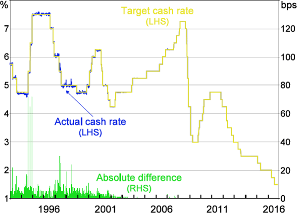
While allowing for a range of interest rates may be necessary in other markets, a well-known feature of the Australian market is that IBOC lending typically occurs with an interest rate equal to the target cash rate. The average daily interest rate on these loans deviated from the target cash rate just 14 times between 2005 and 2010 (each deviation was less than 4 basis points); there have been no deviations since 2010 (Figure 1).
Note: Rounded to nearest basis point
Sources: Authors' calculations; RBA
As a result, capturing IBOC loans in Australia requires a much smaller interest rate range than international studies. This reduces the incidence of false positives, thereby increasing the accuracy of the algorithm (false positives have been a problem for previous applications of Furfine-type algorithms; see Appendix A).
Using 2015 as an example, suppose we restrict the dataset to Furfine-type algorithm matches that imply an interest rate within 100 basis points of the target cash rate, and where the repayment of principal and interest is combined within a single transaction (Figure 2).[17] Then 84.4 per cent of these observations have an implied interest rate equal to the target cash rate. Expanding the range to ±1 basis point around the target captures 84.7 per cent, while a ±5 basis point range captures 85.2 per cent. So expanding the range has little impact on the number of potential loans captured by the algorithm, implying that the incidence of combined-repayment false negatives is low even with an interest rate range of 0 basis points around the target cash rate.
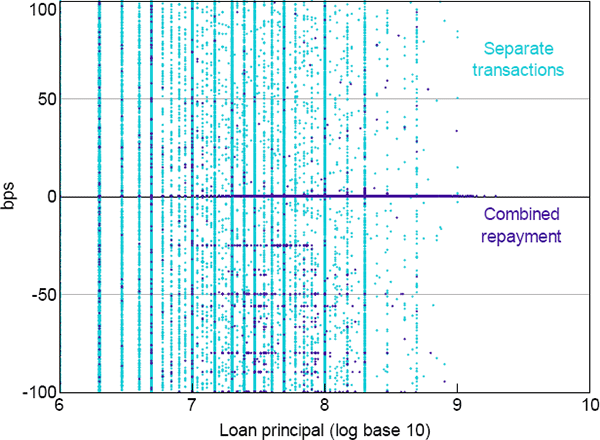
The story is very different when the sample is changed to Furfine-type algorithm matches where the principal is repaid in a separate transaction to interest (Figure 2). There are roughly four times the number of observations relative to the combined-repayment sample, and they are more widely dispersed. This is because there are a large number of small-value payments in our dataset, so there is a high probability of randomly matching two equal-sized payments (i.e. payment and repayment of principal) with a third transaction that would imply an interest rate within 100 basis points of the target cash rate. So, while the large number of small-value payments increases the probability of false positives (relative to the combined-repayment sample), the wide dispersion of the separate transaction observations means the incidence of false negatives could be high with small interest rate ranges (relative to the combined-repayment sample).
The numbers of separate transaction observations captured with implied interest rate ranges of ±1 and ±5 basis points are less than would be expected if none of the separate transaction observations were actually loans but were instead randomly distributed (so we can't statistically rule out the possibility that they are all false positives).[18] However, we can't simply exclude all separate transaction observations, because the number of observations at the target cash rate is significantly above what would be expected if they were false positives.[19]
To summarise, when expanding the allowable interest rate range beyond 0 basis points around the target cash rate, we find small numbers of extra combined-repayment observations, with some of these potentially being false positives. The numbers of extra separate transaction observations at ranges beyond 0 basis points are much larger, but no more than what would be expected if they were all false positives. So we are confident that we are able to minimise the frequency of false positives (by setting an interest rate range of 0 basis points), while still capturing the majority of the IBOC market (i.e. while retaining a low frequency of false negatives).[20]
As noted earlier, while previous international research has discussed the possibility of rollovers, existing algorithms do not attempt to identify them. This is probably because, with sufficiently wide interest rate ranges, it may not be possible to distinguish rolled-over IBOC loans from term lending.[21] Since any term lending captured by the 0 basis point calibration of our algorithm would require these loans to have a term premium of zero and a perfect forecast of future overnight rates, and due to the accuracy of our algorithm's output (see Section 4), we are confident that we are capturing rolled-over IBOC loans rather than term lending.
Given the prevalence of rollovers in the Australian market (see Sections 4 and 5), the ability to identify rollovers (both Furfine-type and credit-facility) is an important innovation to this literature. To the extent that rollovers occur in other countries, the novel features of our algorithm may also improve the identification of overnight interbank loans in these countries. This is particularly the case for countries where low daily interest rate volatility may permit a small interest rate range (such as Canada, see Hendry and Kamhi (2007)).
4. Accuracy of the Algorithm
To evaluate the accuracy of the algorithm, the daily output is aggregated and compared to IBOC Survey data.
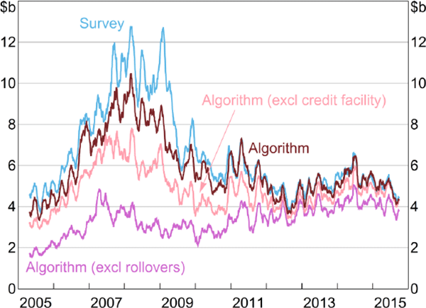
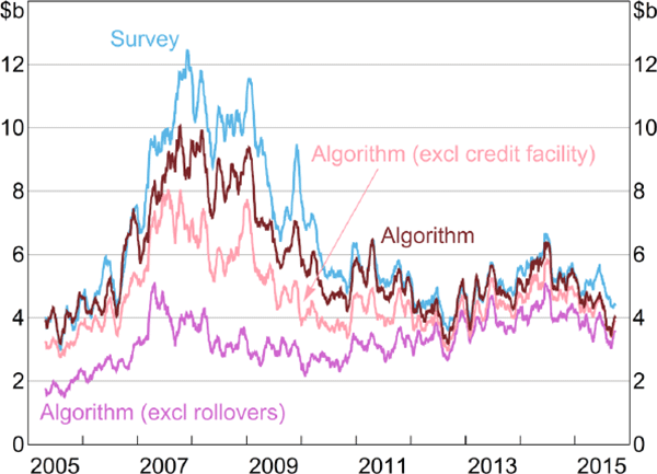
Between 2005 and 2015, the daily correlations between the survey aggregates and the algorithm output are 90 per cent for lending and 92 per cent for borrowing (Figures 3 and 4).[22] As an alternative metric of accuracy (that better accounts for differences in the levels), for both borrowing and lending, our algorithm identifies 89 per cent of the value of IBOC loans between 2005 and 2015.
Note: For days when the institution was included in the survey
Note: For days when the institution was included in the survey
The full algorithm is noticeably more accurate than either the Furfine-type algorithm alone or the algorithm excluding rollovers.[23] The correlations between the Furfine-type algorithm output and the survey aggregates are 75 per cent for lending and 81 per cent for borrowing. Excluding all rollovers further reduces these correlations, to 24 per cent and 37 per cent, respectively (with the proportions of lending and borrowing identified falling to 51 per cent).
The algorithm is also accurate at the individual bank level. For the 22 banks that were included in the survey from early in the sample, over 60 per cent of their daily lending and borrowing correlations are greater than 80 per cent (Figure 5). That said, there are a few banks with very low daily correlations, due to our algorithm not identifying the majority of their IBOC market activity.[24] These low-correlation banks account for only a small share of IBOC market activity (based on the IBOC Survey data), which is why their low correlations have only a small impact on the aggregates discussed above.
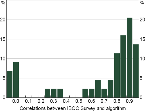
Notes: For days when the institution was included in the survey; horizontal axis by minimum value of bin, bin size of 0.05
It is notable that the algorithm performs very well for the four major Australian banks, with daily lending and borrowing correlations of 96 per cent (Figures 6 and 7).[25] The importance of the credit-facility part of the algorithm is clear in the big spikes in lending between 2006 and 2009. Without the credit-facility part of the algorithm, our algorithm would not have captured these short-term changes in the market.
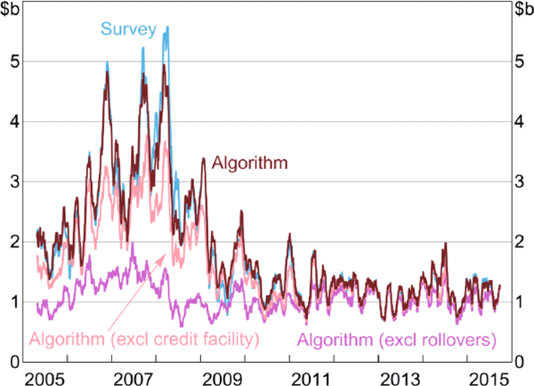
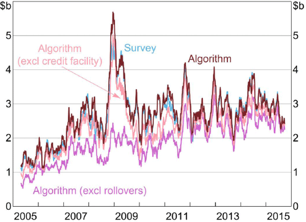
Our algorithm performs well relative to existing studies. This is due to both the algorithm design and the features of the Australian market. With IBOC loans almost always occurring at the target cash rate, we are able to set our implied interest rate range to 0 basis points (around the target cash rate), so there should be very few false positives (some studies exhibit high rates of false positives; see Appendix A).[26] By allowing for rollovers, our aggregate results exhibit high daily correlations with the survey data and identify 89 per cent of the value of all IBOC loans between 2005 and 2015 (the longest time series of any Furfine-type research of which we are aware). This suggests that the incidence of false negatives is comparable to, or lower than, existing studies (see Appendix A).
5. Features of the Market
With the most detailed IBOC market dataset ever constructed now at our disposal, we explore several features of the market that were previously unobservable. The results in this section both improve our understanding of how the market functions, and help to explain several of the changes that have occurred over the past decade.
With this paper being the first to identify rollovers, we start by determining the incidence of rollovers and whether rollovers and non-rolled loans exhibited different trends over the past decade (Section 5.1). Given that we find very different trends, we seek to determine whether rollovers and non-rolled loans are used for the same purpose and some reasons why they may not be perfect substitutes. We find that, while both loan types appear to be used to satisfy banks' late-day funding needs, the fact that rollovers are conducted earlier in the day (when banks may be less certain of their late-day funding requirements) is one reason why they may not be perfect substitutes (Sections 5.2 and 5.3).
We decompose the timing of IBOC market activity based on bank type, and determine whether the timing of banks' IBOC market activity has changed over the past decade (Section 5.2); we pay particular attention to the period following the introduction of same-day settlement of direct entry obligations. We find that banks are currently managing their end-of-day ESA balances during a briefer period (towards the end of the day) than has been the case historically.
We use regression techniques to determine when banks agree to a loan (as opposed to when it is settled in RITS; Section 5.3). Knowing agreement times is important for operational decisions made by the RBA. For example, the optimal timing of late-day open market operations depends on the timing of IBOC market activity. And it is important to know the periods during which a delay of high-value payments could affect the IBOC market.[28]
Finally, we decompose the changes in IBOC market activity into changes in the average size of loans and changes in the number of loans (Section 5.4; such a decomposition was not possible prior to the construction of our loan-level database). And we highlight the surprising fact that banks calculate the interest on rollovers using simple interest (as opposed to compounding), even though daily interest typically remained outstanding for the life of the rollover (Section 5.5).
5.1 Incidence of Rollovers
Rollovers appear to have been more common historically than in recent years, accounting for almost half of daily IBOC lending during 2008, before falling to around 10 per cent recently (Figure 8). Over the entire sample, 72 per cent of individual rollovers (i.e. those identified by the Furfine-type algorithm) and credit-facility rollovers had been rolled for less than five trading days.
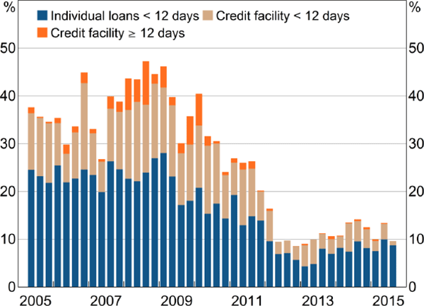
Notes: Share of algorithm-identified lending; excluding weekends and public holidays
As noted earlier, market liaison indicated that risk limits may prevent loans from being rolled over for an extended period. Our results suggest that while this may be a good characterisation of current practice, this was not always the case, with some credit-facility-type loans being rolled over for more than two months before any interest was paid.
Looking at the values of rollovers and non-rolled loans, the halving of market activity since the beginning of 2009 (shown in Figures 3 and 4) mostly involved a fall in the value of rollovers (Figure 9). The average value of IBOC lending during 2015 was 48 per cent smaller than at the beginning of 2009. This fall comprised an 87 per cent fall in the average value of rollovers and a 13 per cent fall in the average value of non-rolled loans.
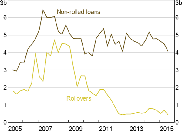
In Section 5.3, we discuss some reasons why rollovers and non-rolled loans may not be perfect substitutes. But the cause of the fall in rollovers is unknown, and a detailed analysis is left for future research.
5.2 Timing of IBOC Transactions
RITS is open for settlement from 7.30 until 22.00, but the trading day is split into several ‘sessions’, with different rules governing each session (RBA 2015a). For the purposes of our research, it is sufficient to focus on just three of the sessions (Day, Close and Evening).
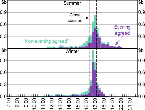
The ‘Day’ session finishes at 16.30, at which point new SWIFT customer payments are no longer accepted (customer payments already entered into RITS may be settled in a later session). The ‘Close’ session, operating from 16.30 until 17.15, then allows banks to borrow/lend ESA balances before some banks are able to exit the market.
The ‘Evening’ session opens at 17.20. All ‘evening agreed’ banks must remain available to settle RITS transactions during this session. All SWIFT payments (not just customer payments) involving a ‘non-evening agreed’ bank, and all non-bank Austraclear payments (that are settled via banks' ESAs), must settle before the end of the Close session. As a result, non-evening agreed banks have the option, but are not required, to operate during the Evening session (via cash transfers or Austraclear, not SWIFT). This means that any uncertainty surrounding non-evening agreed banks' end-of-day ESA balances is likely to dissipate earlier in the trading day than it does for evening agreed banks.
During Australian Eastern Standard Time (winter), all SWIFT settlements finish by 18.30; SWIFT settlements can occur until 20.30 during Australian Eastern Daylight Time (summer).[29] As a result, the intraday distribution of RITS transactions (including IBOC loans) differs between summer and winter months.
The algorithm output revealed the following features about the timing of non-rolled loans (these include the first days of loans that are subsequently rolled over; Figure 10):
- There is very little non-rolled lending until late in the day, when banks are more certain of their end-of-day ESA balances.
- Non-evening agreed banks are a party to a higher proportion of Day session loans (50 per cent) relative to the Close and Evening sessions (32 and 16 per cent, respectively). This is expected because certainty about their end-of-day positions occurs earlier in the day.
- The majority of non-rolled lending settles during the Close session.
Notes:
Time of first-leg transactions, including increase in principal for credit-facility
loans
(a) Loans for which at least one participant is a non-evening agreed bank
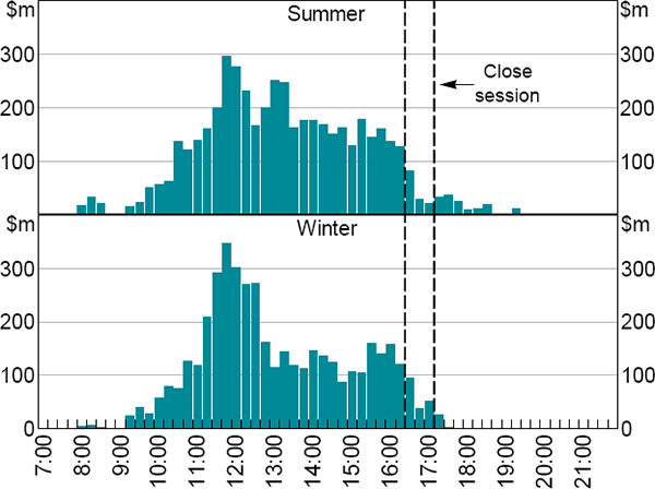
In contrast to first-leg transactions, repayment transactions settle throughout the Day session (Figure 11).
Note: Time of all second-leg transactions, including decrease in principal for credit-facility loans
5.2.1 Changes over time
The share of non-rolled lending that settles during the Close session has increased over time (from 48 per cent in the 2006 winter season to 62 per cent in the 2015 winter season), with a corresponding decrease in both the Day and Evening sessions (Figure 12).[30] This suggests that banks are managing their end-of-day ESA balances during a briefer period than has been the case historically.
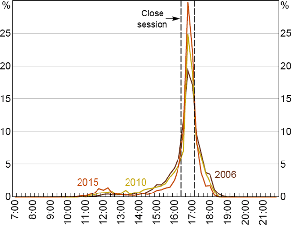
Note: Time of all first-leg transactions
From 25 November 2013, the RBA enhanced RITS to provide for same-day settlement of direct entry obligations in several batches (these transactions were previously settled in a single batch at the beginning of the following business day). With the majority of non-rolled IBOC market activity occurring late in the day, batches that settle early in the day were not expected to affect the IBOC market. Similarly, batches that settle after 16.45 do not affect the IBOC market, because the RBA has implemented alternative arrangements for the settlement of these batches (Fraser and Gatty 2014; RBA 2015c).
That leaves the 16.45 batch as potentially affecting the IBOC market. Although the 16.45 batch settles after one-third of non-rolled IBOC loans had historically already settled, banks have information on the size of this batch before 16.15. As a result, banks' uncertainty about their end-of-day ESA balances, at times when the majority of non-rolled IBOC activity had historically occurred (i.e. the Close and Evening sessions), was not expected to change following the introduction of same-day settlement. So the 16.45 batch was not expected to further delay market activity.
The data is consistent with this expectation. While there was an increase in the proportion of Close session settlements between 2012 and the period immediately following the introduction of same-day settlement (from 38 to 42 per cent; Figure 13), a two-sample Kolmogorov-Smirnov test is unable to reject (at the 10 per cent significance level) the null hypothesis that the 2012 and 2013 distributions are the same. Moreover, this increase is consistent with the trend increase in Close session settlements discussed above. And the corresponding decrease in the share of settlements mainly occurred in the Evening session, which is inconsistent with the 16.45 batch causing a delay in market activity.
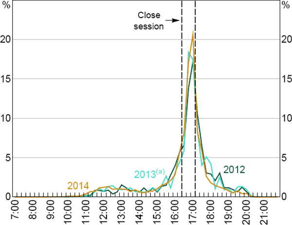
Notes:
Time of all first-leg transactions
(a) 25 November–31 December only
5.3 Timing of Rollovers and Non-rolled Loan Agreements
Knowing the time of day at which rollovers are typically agreed may help to explain why the value of rollovers has declined so dramatically since 2009 while non-rolled loans have remained broadly stable (Figure 9). However, since rollovers do not have a corresponding RITS transaction on each day they are rolled, it is not possible to determine the time of day at which each rollover is agreed. Nevertheless, since the IBOC Survey asked respondents to split their gross lending/borrowing figures into the trading sessions in which the loans were agreed, we can estimate the sessions in which rollovers are typically agreed by comparing the algorithm-identified value of daily rollovers to the survey data over time (using regression techniques).[31]
Knowing agreement times is also important for operational decisions made by the RBA (as was discussed at the beginning of Section 5). And it is possible that non-rolled loans may be agreed in one session and settled in another (the analysis in Section 5.2 is based on settlement time rather than agreement time). Our regression analysis is also able to estimate the typical share of non-rolled loans agreed in one session and settled in another.
If there were no rollovers and the algorithm were 100 per cent accurate, we would be able to determine the exact value, every day, of IBOC loans agreed in one session and settled in another (by comparing the survey data to the algorithm output for each session). The regression analysis is required because random changes in the agreement time of rollovers, and loan-identification errors from the algorithm (i.e. false positives and negatives), confound our ability to identify daily differences in agreement and settlement times.
Moreover, the potential size of these confounding factors is likely to vary with the value of IBOC market activity (e.g. the value of false negatives is limited by the true value of lending), causing conditional heteroskedasticity. And random changes in the agreement time of rollovers would be negatively correlated across sessions (i.e. a higher than expected share of rollovers in one session necessitates a lower than expected share in another session).
For these reasons, we implement our regression analysis using a three-equation (one for each session) seemingly unrelated regression (SUR) model with conditional heteroskedasticity.[32] The model is:
where:
- i = Day (1), Close (2), or Evening (3) sessions
- t = trading day
- diffi,t = difference between the value of loans agreed in session i of day t (from the IBOC Survey) and the algorithm-identified value of non-rolled loans[33] settled in session i of day t
- rollt = value of rollovers (identified by the algorithm) in day t
- nrt = value of non-rolled loans (identified by the algorithm) in day t
- ui,t = residual component of diffi,t; modelled as a first-order autoregression
- εi,t = unexplained component of ui,t (assumed to be a random draw from a multivariate normal distribution)
- ωi,t = conditionally-heteroskedastic variance of εi,t
- ci,j = contemporaneous correlation between εi,t and εj,t
-
 are the parameters to be estimated for each session
i.
The remainder of this section provides interpretations for the parameters of interest, explains some potential biases that may hamper estimation, details the estimation results, and discusses the implications of these results. A formal derivation of the model's functional form and the asymptotic properties of the parameter estimators are given in Appendix D.
5.3.1 The parameters of interest and potential biases
Starting from Equation (1), suppose, for the moment, that the following conditions hold:
- no loan-identification errors;
- the shares of rollovers agreed in each session are constant over time; and
- the shares of non-rolled loans agreed in one session and settled in another are constant over time.
Then αi + ui,t = 0 for all i and t. This is because, in this scenario, diffi,t has just three components: rollovers agreed in session i, plus non-rolled loans agreed in session i but settled in a later session, minus the value of non-rolled loans settled in session i that were agreed in a previous session. And with these three components being a constant share of the daily aggregates (in this scenario), diffi,t = βirollt + γinrt for all i and t.
Moving away from this stylised scenario, diffi,t = βirollt + γinrt does not hold due to loan-identification errors, changes in the per session shares of daily rollovers, and changes in the per session shares of daily non-rolled loans that are agreed and settled in different sessions. All of these components are captured in αi + ui,t; with ρiui,t − 1 capturing the persistence in these components, αi capturing the mean, and εi,t being the unexplained portion of these components.[34]
Therefore, given what this section seeks to determine, the parameters of interest and their interpretations are:
- βi – the typical share of daily rollovers agreed in session i; and
- γi – the typical share of daily non-rolled loans agreed in session i and settled in a later session, minus the typical share settled in session i that was agreed in an earlier session.
Because the shares of daily rollovers agreed in each session must sum to 100 per cent, random changes in these shares induce negative correlations between the session-specific shocks (εi,t). Random changes in the share of daily non-rolled loans agreed in session i and settled later minus the share settled in session i that was agreed earlier' (henceforth, ‘net share’) also induce negative correlations. For example, a reduction in the share agreed in Session 1 and settled in Session 2 would reduce the Session 1 net share but increase the Session 2 net share. This is why a SUR framework is used (i.e. why non-zero ci,j parameters are allowed).
As long as these random changes in shares are independent of the daily values of rollovers and non-rolled loans, these random changes will not cause our parameter estimators to be inconsistent (see Appendix D). However, the impact of these random changes on the variances of the session-specific shocks (ωi,t) will depend on the daily values of rollovers and non-rolled loans, which is why we incorporate conditional heteroskedasticity into our model (see Appendix D).
Unfortunately, our parameter estimators will be inconsistent if the loan-identification errors are correlated with the daily values of rollovers or non-rolled loans (see Appendix D). Such correlation is a reasonable assumption given that the value of false negatives on any day is bounded by the true value of lending.[35] However, given the accuracy of our algorithm, we do not expect any inconsistencies to be large.
To potentially help attenuate any estimator inconsistency, we impose theory-based restrictions on the βi parameter estimators. First, since rollovers must be agreed at some point during the day, the sum of the shares agreed in each session must equal 1 (i.e. ∑iβi = 1). Second, rollovers cannot reduce the difference between the IBOC Survey and algorithm output (i.e. βi ≥ 0 ∀ i).[36]
5.3.2 Estimation results
Table 2 shows the βi parameter estimates produced by maximum likelihood estimation of the model (with the aforementioned restrictions) for four datasets: the lending/borrowing of the major banks, and the lending/borrowing of the 18 other banks that were included in the IBOC Survey from early in the sample.[37] The results suggest that rollovers are typically agreed in the Day session. This is not surprising given that the majority of repayments occur during the Day session (Figure 11), and rollovers would need to be agreed before repayment was due.
While almost all of the rollovers to which the major banks are a party are typically agreed in the Day session, more than 10 per cent of the other banks' rollovers are typically agreed in the Close session. The hypothesis that all rollovers are agreed in the Day session is statistically rejected at the 5 per cent level for all four regressions in Table 2.
| Day | Close | Evening | |
|---|---|---|---|
| Major banks' lending | 98 (102) | 0 (−4) | 2 (5) |
| Major banks' borrowing | 96 (91) | 3 (2) | 1 (1) |
| Other banks' lending | 83 (81) | 16 (16) | 0 (0) |
| Other banks' borrowing | 86 (78) | 11 (10) | 4 (3) |
For the major banks, the theoretical restrictions are statistically rejected by the data (at the 1 per cent level); the unrestricted estimates are given in parentheses in Table 2. Given that the restrictions must hold with the true parameter values, the fact that they are statistically rejected suggests our concerns about estimator inconsistency are well-founded. That said, the differences between the restricted and unrestricted estimates would not change our qualitative conclusions, so the inconsistency is not qualitatively important (as expected). For the other banks, likelihood ratio tests of the theoretical restrictions produce p-values of 0.90 for lending and 0.09 for borrowing.
With the γi parameters representing the typical ‘net shares’, the γi parameters would sum to zero (in the limit) in the absence of estimator inconsistencies. As shown in Table 3, the sum is less than zero for three of the four regressions, suggesting that, for at least some sessions, loan-identification errors are negatively correlated with the value of identified non-rolled loans.
| γi parameters Per cent |
Correlations (ci,j) |
|||||
|---|---|---|---|---|---|---|
| Day | Close | Evening | Sum | Day/Close | Close/Evening | |
| Major banks' lending | 2 | 18 | −25 | −5 | −0.15 | −0.77 |
| Major banks' borrowing | 6 | 15 | −24 | −3 | −0.32 | −0.79 |
| Other banks' lending | 11 | 0 | −17 | −6 | −0.34 | −0.61 |
| Other banks' borrowing | 20 | −7 | −12 | 1 | −0.36 | −0.28 |
Assuming the correlations between loan-identification errors and identified non-rolled loans have the same sign in every session, the estimated γi parameters can still be used to provide a range for the estimated proportion of non-rolled loans typically agreed in the Close session and settled in the Evening session.[38] For the major banks, this range is 20–25 per cent for their lending and 21–24 per cent for their borrowing. For the other banks, the range is 11–17 per cent for their lending and 12–13 per cent for their borrowing.[39]
Since 45 per cent of the major banks' non-rolled lending, and 37 per cent of their non-rolled borrowing, settles in the Evening session (on average over the sample), these results suggest that the majority of this lending/borrowing was actually agreed in the Close session. This means that 75–87 per cent of the major banks' non-rolled lending/borrowing is estimated to have been agreed before the end of the Close session. This proportion is 91–99 per cent for the other banks.
As expected, the session specific shocks (εi,t) are negatively correlated between consecutive sessions (Table 3), while the correlations between non-consecutive sessions are close to zero (with absolute values less than 0.03).[40] The conditional heteroskedasticity (i.e. the τi and φi parameters in Equation (4)) is estimated to be statistically significant (at the 1 per cent level) in all four regressions.
5.3.3 Implications of these results
Combining the results presented above with those from Section 5.2 suggests that rollovers are typically agreed earlier in the day than non-rolled loans (when banks may be less certain of their late-day funding needs). However, rollovers still appear to be used by banks to manage their end-of-day ESA balances. If a bank lends via a rollover, the probability of that bank also lending via a non-rolled loan on that day is 75 per cent, while the probability of borrowing via a non-rolled loan is just 42 per cent.[41] The conditional probabilities when borrowing via rollover are similar, with the probability of non-rolled borrowing at 76 per cent, and non-rolled lending at 40 per cent.[42]
With banks appearing to use both rollovers and non-rolled loans to manage their end-of-day ESA balances, the fact that the majority of the fall in rollovers (between 2009 and 2015) occurred while non-rolled loans remained broadly steady suggests that the cause of the fall in rollovers is unlikely to be a fall in generic late-day funding needs. For example, Hing, Kelly and Olivan (forthcoming) suggest that the fall in rollovers may be due to a fall in precautionary demand for ESA balances, with this precautionary demand satisfied via rollovers.
Moreover, there may be other reasons (beyond time of day) why rollovers and non-rolled loans may not be perfect substitutes (such as the increasing credit risk with each day it is rolled over).[43] So it may be a feature of rollovers that has led to the fall. The first port of call will be to determine whether the fall in rollovers corresponds with increased activity in other markets (such as the term or secured lending markets).
5.4 Number and Average Value of Loans
Over the entire sample, quarterly changes in the average number of loans per day and changes in the average value of these loans have been roughly equal contributors to the changes in the value of IBOC loans (Figure 14).[44]
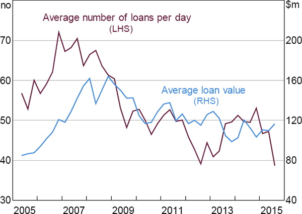
The fall in the average number of loans per day is mainly composed of a fall in the average number of rollovers, with the average daily number of non-rolled loans at the end of the sample (33) being little changed from the beginning (36). Until 2009, the average sizes of rollovers and non-rolled loans were essentially the same (the average absolute difference during this period was just 8 per cent of the level). As the number of rollovers fell, the remaining rollovers were typically smaller than the non-rolled loans ($78 million versus $123 million, respectively).
5.5 Simple Interest for Rollovers
Of the 96,052 first-leg transactions the Furfine-type algorithm identifies as being part of an IBOC loan, only 9 were repaid with compound interest (with these potentially being false positives). Instead, the interest owed on rollovers is almost always calculated using simple interest. For example, a loan rolled over from Monday to Thursday is repaid as principal plus 3 times daily simple interest. This means that when calculating repayments on rollovers, lenders are not accounting for any interest that was owed to them throughout the rollover period; in other words, borrowing banks that roll over are essentially receiving small interest-free loans.[45] With several banks borrowing more than double the amount they lent (between 2005 and 2015), this lack of compounding has benefited some banks more than others.
6. Conclusions and Future Research
The aim of this paper was to construct a loan-level database of IBOC loans to improve the information available to the RBA about how this pivotal market has historically functioned. To this end, we designed an algorithm to identify IBOC loans using a census of payments settled through Australia' high-value payments system.
While algorithms for this purpose already exist in the literature, we found that these existing algorithms failed to identify the majority of IBOC loans in Australia. This is because these algorithms do not attempt to identify rollovers.
Many rollovers were identified by extending existing algorithms to recognise the features of rollovers (such as principal repayments that do not occur the following day, and multiple days' worth of interest either paid in one transaction or over several days). The success of these extensions was aided by the low interest rate volatility in the Australian IBOC market, which allowed us to calibrate our algorithm with a smaller interest rate range than is typical in the literature (thereby minimising the frequency of false positives).
With existing algorithms only matching pairs of transactions (i.e. the original loan and the repayment), identification of rollovers that exhibit features more akin to a credit facility required the development of an algorithm that is fundamentally different to the Furfine-type algorithms that exist in the literature.
The combination of the extended Furfine-type algorithm and credit-facility algorithm was very successful in identifying Australian IBOC loans. Between 2005 and 2015, the daily correlations between the aggregated survey data and the algorithm output are greater than 90 per cent (increasing to 96 per cent for the major banks). Such accuracy is uncommon in the existing literature, which is potentially due to both the inability of existing algorithms to identify rollovers and the larger interest rate ranges required for algorithms used in other jurisdictions.
Using the loan-level database, we find that the halving of market activity between 2009 and 2015 mainly involved an 87 per cent fall in rollovers (rollovers accounted for almost half of the market before the fall). We also find that while both rollovers and non-rolled loans appear to be used to satisfy banks' late-day funding needs, they are not perfect substitutes, with rollovers conducted earlier in the day (when banks may be less certain of their late-day funding requirements).
Given the detail and accuracy of the algorithm output, previously infeasible research projects are now possible, such as forthcoming analysis of how the market changed during the global financial crisis. Moreover, the algorithm could be modified to capture secured or long-term interbank lending, providing the same level of detail about these markets as has been shown here for the IBOC market, and could also be adapted for use in other countries.
Appendix A: Literature Review
The first part of our algorithm is based on the work of Furfine (1999) and other papers that have followed a similar procedure. A number of papers have assessed the accuracy of Furfine-type algorithms, with varying results.
Access to transaction-level data where interbank loans are flagged appears to be rare. Armantier and Copeland (2015) use data from two US banks that unilaterally insist on marking these transactions as loans, and find that the algorithm performs poorly: on average, 81 per cent of transactions identified as loans were not actually loans (false positives or Type I errors), while the algorithm failed to pick up 23 per cent of loan-related transactions (false negatives or Type II errors).
Guggenheim, Kraenzlin and Schumacher (2011) and Arciero et al (2016) use transaction-level data, from Switzerland and the euro area, respectively, to assess the accuracy of their algorithm. Although these studies are based on different markets, and are therefore not directly comparable, both report lower Type II error rates than Armantier and Copeland – 10 per cent and 1–9 per cent, respectively. However, while neither European study assesses Type I error rates at the transaction level, the euro area algorithm identifies well over 100 per cent of the daily overnight trading reported by EONIA panel banks (inter-quartile range of 120–160 per cent), suggesting that Type I errors may be a problem.
More commonly, papers use aggregated filings by banks at the end of the day (or end of the quarter) to assess the accuracy of their algorithms. These data are typically aggregated gross or net lending reported to the central bank for regulatory purposes or for data construction (akin to the RBA's IBOC Survey). For example, Akram and Christophersen (2013) find that their algorithm accurately identifies aggregate daily lending for the majority of the banks in their Norwegian sample (similar to our results), but that large discrepancies for a few banks cause an average absolute daily deviation (aggregating across all banks) of 20 per cent (ours is 13 per cent).
Interestingly, Kovner and Skeie (2013) compare this method of accuracy determination to that of Armantier and Copeland (2015), and find that they do not square – using quarterly aggregated regulatory filings suggests a higher degree of accuracy than transaction-level comparisons. There are many reasons why this may occur. For example, Armantier and Copeland only look at the accuracy of loans involving two banks, whereas Kovner and Skeie look at the entire federal funds system. Moreover, some banks may transact on behalf of other client banks, so some of the false positives found by Armantier and Copeland may actually be loans but are assigned to the wrong bank (the banking system aggregates would be unaffected).
A different approach was taken by Millard and Polenghi (2004), who assess the accuracy of a Furfine-type algorithm by comparing the daily average of implied interest rates across all identified loans with the daily SONIA rate. Based on this metric, their algorithm performs very well (a daily correlation of 97 per cent). However, while this suggests that false positives are unlikely to be a problem, this method cannot elucidate the volume of false negatives (e.g. these excluded loans may have the same average interest rate as the captured loans).
In Australia, Sokolov et al (2012) use a week (in February 2007) of RITS data and a Furfine-type algorithm to identify interbank loans. With only a week of data, their algorithm only allows for overnight and very short-term loans.[46] Given the high share of rollovers during this period, not accounting for rollovers leads to a high rate of false negatives (65 per cent of the IBOC loans identified by our algorithm).
By allowing non-rounded transactions to be loans, Sokolov et al may also be capturing secured overnight loans. This may be why, even with a high false negative rate, their identified overnight loans represent 126 per cent of the IBOC market.
Appendix B: Detailed Description of the Algorithm
This appendix details the Furfine-type and credit-facility algorithms.
Before our algorithm begins, any transactions involving institutions that are known to not participate in the IBOC market are removed from the dataset, along with any transactions where the paying and receiving parties are the same.
Several parameters must be calibrated before running the algorithm (these are underlined in the following description).
B.1 The Furfine-type Algorithm
This part of the algorithm identifies transactions that could feasibly be considered the ‘first’ (initial payment) and ‘second’ (repayment) legs of an IBOC loan. It is implemented in Stata, using data from both RITS cash transfers and the Austraclear feeder system. There were 7,386,289 transactions between 4 January 2005 and 15 January 2016.
Step 1 Consider only rounded transactions as possible first legs of a loan (the baseline algorithm uses a minimum of $1 million, increasing in increments of $1 million). 919 687 transactions identified.
Step 2 Match up potential first legs with all possible second legs: any transaction between the same counterparties (but going in the reverse direction) occurring at any point within a set repayment period (the baseline algorithm searches over the following 15 days). 183 183 418 possible matches generated.
Step 3 Calculate a plausible range of interest payments as defined by the calibrated range of interest rates (the baseline algorithm has a range of 0 basis points around the target cash rate) and accounting for any changes in the target cash rate:[47]
- single-day simple interest range = principal × [cash rate ± range]
- multiple-day simple interest range = single-day simple interest range × number of days since first leg
- compound interest range = principal × [{(1 + [cash rate ± range]) ^ number of days} − 1].
Step 4 Identify matches associated with full repayment on one day:[48]
- a single match with a second leg equal to principal + cumulative interest (simple or compound); or
- two matches (with the same first leg) – one with a second leg equal to principal, the other with a second leg equal to the cumulative interest payment.
Step 5 Identify matches (with the same first leg) that could be part of a rollover. These include matches with second legs equal to:
- repayment of principal along with an interest payment that does not cover multiple days (this interest payment can be combined with the principal or in a separate match); and
- daily interest payments (where these occur on days between the first leg and the date the principal is repaid).
Step 6 Drop all matches not identified in Steps 4 or 5. 151 801 possible matches remain.
Step 7 Drop any potential loans that have a repayment structure identified in Step 5 but do not have associated matches that sum to at least the necessary cumulative interest payments as calculated in Step 3. 102 802 possible loan sets remain.[49]
Step 8 If multiple matches exist for a first leg (i.e. a first leg is matched with several independent second legs – ‘independent’ means matches that are not all part of the same loan set as identified in Steps 4 or 5):
- Keep the matches associated with loan sets that represent the shortest rollover length. 102 696 possible loan sets remain.
- If multiple matches remain (i.e. loan sets with the same rollover length), keep the matches for the loan set with the interest payment that is closest to the centre of the calculated range.[50] 102 696 possible loan sets remain.
- If multiple matches remain, the loan sets must be identical (with respect to the value, term and interest rate, but not necessarily the repayment structure). So only the loan set associated with the first match processed by the algorithm is kept (this choice is arbitrary). 101 420 possible loan sets remain.
Step 9 At this point, each remaining first leg will be associated with a single loan set. But a second-leg transaction may still be matched with multiple first legs (i.e. as a second leg in multiple loan sets) – if so, only the match associated with the final first leg is kept (i.e. the second leg is associated with the most recent loan set). 101 274 possible loan sets remain.
Step 10 If a transaction appears as both a second leg and a first leg (in different loan sets), keep only the match where it is identified as a second leg (this choice is arbitrary). 100 269 possible loan sets remain.
Step 11 For all of the matches dropped in Step 9, the algorithm checks whether the first legs could be matched with a different (and as yet unmatched) second leg (such a match would have been dropped at Step 8). It does this by re-running the algorithm excluding all the matches that remain after Step 10. 100 315 loan sets identified.
Since rollovers are actually consecutive overnight loans (without the corresponding RITS transaction), when calculating loan values, the algorithm counts rollovers as a new overnight loan on each day prior to the repayment of principal (except on weekends and public holidays).
B.2 The Credit-facility Algorithm
This part of our algorithm is implemented in Matlab, using data from RITS cash transfers and excluding transactions that are part of any matches identified from the Furfine-type algorithm.
Step 1 Construct a three-dimensional array of gross daily ‘payments’. ‘Payments’ include all transactions that are greater than the minimum transaction size and that are a multiple of the calibrated increment. Cell (i,j,t) of this array will equal the sum of all payments going from Bank i, to Bank j, on day t.
Step 2 The key variable in the credit-facility algorithm is the ‘potential outstanding’ loans on each day and between each pair of banks. That is, the sum of all lending by Bank i to Bank j that is still outstanding on day t. So the ‘potential outstanding’ array has identical dimensions to the array created in Step 1.
Step 3 For t = 1, and for all i and j, if the payments from Bank i to Bank j exceed those from Bank j to Bank i, the payments from Bank i to Bank j minus those from Bank j to Bank i are entered into the potential outstanding array as the potential outstanding loans from Bank i to Bank j at t = 1. Otherwise, the entry in this cell is zero.
Step 4 For each day t > 1, and for all i and j:
- Compute the daily maximum and minimum interest on potential outstanding loans from Bank i to Bank j by multiplying the relevant potential outstandings at the end of the previous day by the target cash rate on the previous day, plus/minus the range of interest rates.[51]
- The maximum and minimum amounts of day t interest outstanding are equal to the above constructed daily interest amounts plus the maximum and minimum (respectively) values of interest still outstanding from the previous day (which could be zero).
-
Search for any transactions on day t that go from Bank j to Bank
i and that are equal to either:
- an amount in-between the day t maximum and minimum interest outstanding;
- an amount in-between the maximum and minimum interest outstanding plus the principal outstanding on loans from Bank i to Bank j (from the potential outstanding array) at the end of the previous day; or
- an amount in-between the maximum and minimum interest outstanding, plus part of the principal outstanding (which must be a multiple of the calibrated increment) on loans from Bank i to Bank j at the end of the previous day.
-
If such a transaction is found:[52]
- In all cases, the interest outstanding (both maximum and minimum) between Banks i and j, on day t, is set to zero.
- When the transaction equals principal plus interest, the remaining principal outstanding on loans from Bank i to Bank j is zero. So the day t potential loans outstanding from Bank i to Bank j is just equal to the relevant day t payments (so the potential outstanding array is updated in the same manner as Step 3, just with a different t).
-
When the transaction equals the interest payment only, or with partial principal
repayment, the potential outstanding array is updated as follows.
-
Suppose Bank i's potential outstanding loans to Bank j
from the previous day, plus the day t payments (from Step 1) that
go from Bank i to Bank j, minus any partial principal
repayment, are greater than the equivalent sum going from Bank j to
Bank i. Then Bank i's potential outstanding loans to
Bank j on day t are equal to:
where ‘PotOut’ is the potential outstanding array, ‘Pay’ is the payments array, ‘Prin’ is the principal component of the repayment transaction (if applicable). - Otherwise, Bank i's potential outstanding loans to Bank j on day t are equal to zero.[53]
-
Suppose Bank i's potential outstanding loans to Bank j
from the previous day, plus the day t payments (from Step 1) that
go from Bank i to Bank j, minus any partial principal
repayment, are greater than the equivalent sum going from Bank j to
Bank i. Then Bank i's potential outstanding loans to
Bank j on day t are equal to:
- If no interest payment transactions are found at Step 4c, and the last day at which the interest owed to Bank i from Bank j was reset to zero (Step 4di) is more recent than t minus the calibrated repayment period (90 days for the baseline calibration), then the relevant cell in the potential outstanding array is updated in the same way as Step 4diii.[54]
- However, if no interest payment transactions are found at Step 4c, and the last day at which the ‘interest owed to Bank i from Bank j’ was set to zero is equal to t minus the calibrated repayment period (henceforth t − c), then the algorithm sets the potential outstanding loans owed to Bank i from Bank j on day t − c equal to zero (in the potential outstanding array), and re-runs Steps 4a–4e for Banks i and j on all days between t − c and t (inclusive).[55]
Step 5 If a repayment transaction is either interest-only or a partial principal repayment, the remaining principal must form part of a new loan (that is eventually repaid). This step removes any potential outstandings where this is not the case.
Step 6 At this point, the potential outstanding array will only include payments that have identified repayments at some point within the set repayment period, and where the principal is either repaid in full or forms part of a new loan. So this array will be a summary of outstanding credit-facility-type loans between each bank and on each day during the sample period.
Our algorithm output required some adjustments before analysis could be undertaken:
- With a repayment period of 15 days for the Furfine-type algorithm, the first 15 days of our sample and the last 15 days of our sample may not capture all loans outstanding on these days (e.g. if the first-leg transaction of a rollover occurs before the beginning of our sample or a second-leg transaction occurs after the end of our sample). Similarly, the credit-facility algorithm may incorrectly eliminate IBOC transactions within 90 days of the beginning of our sample, and will not be able to eliminate non-IBOC transactions that occur within 90 days of the end of our sample. As a result, all analyses in this paper are conducted on a truncated sample of 5 April 2005 to 16 October 2015 – of the 100,315 loan sets identified by the Furfine-type algorithm, 96,052 occur during this period.
- Since intra-group loans are explicitly excluded from the IBOC Survey, we removed IBOC loan transactions between banks known to have merged during our sample period (only transactions after the merger date were removed).
Appendix C: Expanding the Interest Rate Range
This appendix provides some information on the impact of expanding the interest rate range beyond zero (as is done in the existing literature).
Allowing for a ±1 basis point range in the Furfine-type algorithm slightly improves the correlation of aggregate lending between the survey data and algorithm output (from 90 per cent to 91 per cent). However, this may be driven by an unrelated level effect rather than actually capturing more IBOC loans.
To explain, expanding the range captures more loans during the 2007–09 period (when our algorithm is least accurate) than during other periods, which improves the correlations and the proportions of loans identified (Figures C1 and C2). However, after extracting the level effect, the daily lending correlation is lower with a ±1 basis point range than with a 0 basis point range (by 0.36 percentage points), while the borrowing correlation only marginally increases (by 0.02 percentage points).[56] Moreover, expanding the range worsens the major banks' lending and borrowing correlations and increases the proportions of loans identified for the major banks to over 110 per cent (from 101 and 104 per cent, respectively).[57]
It is possible that, in expanding the range, we are capturing some other form of lending (term lending, for example), and that it is just a coincidence that the increase in this lending occurred at the same time as our algorithm's accuracy fell.
Allowing for a ±5 basis point range unambiguously worsens the algorithm's fit relative to the ±1 basis point range.
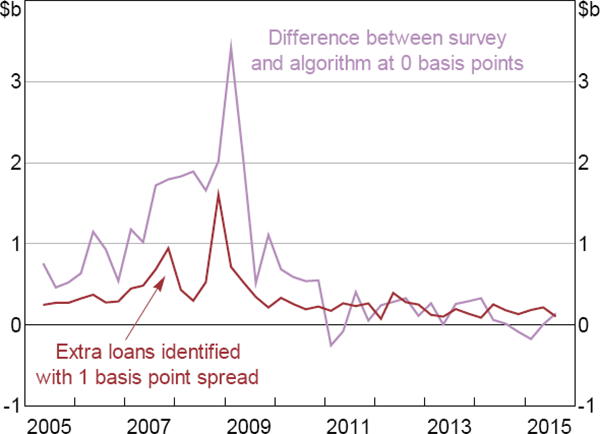
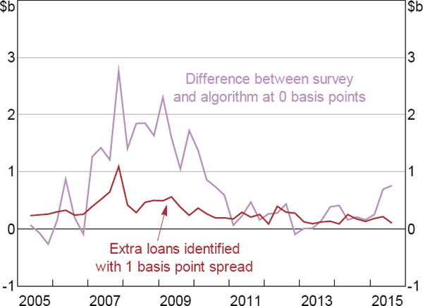
Appendix D: Derivation of the Model
For simplicity, this appendix assumes that there are no rollovers and that there is no persistence in ui,t. The intuition when rollovers and persistence are included is the same. Suppose the true data-generating process is (where γi,t is the ‘net share’ in session i of day t):
With the net share varying over time, ui,t consists of loan-identification errors only. However, suppose we estimate:
Then, by combining Equations (D1) and (D2):
Estimating a constant net share causes the conditional variance of  (conditional on nrt,
  and
and  to differ from the variance that does not condition on nrt:
Assuming changes in γi,t are independent of both nrt and ui,t:
Equation (D4) justifies the functional form we assume for the conditional heteroskedasticity in our model.
Now suppose the parameters are estimated using ordinary least squares (OLS). By construction,
the estimated sample covariance between nrt and  will be zero. Assuming the conditions required for the weak law of large numbers hold, the
sample covariance converges in probability to the population covariance. Therefore, the
following holds for the population covariance:
Which, using Equation (D3), can be rewritten as:
If γi,t and nrt are independent, then the population covariance can be expanded to:
Using Equations (D5) and (D6), and re-arranging, gives the following limit value for  (i.e. as T → ∞, where T is the sample size):
So, in the limit, the OLS estimator of the constant net share ( )
will equal the mean of the net share plus a bias term caused by any correlation between
non-rolled loans and the loan-identification error.
If the bias term is non-zero, then an estimator for  that
accounts for the conditional heteroskedasticity of
  (such as
the Gaussian maximum likelihood estimator (MLE) used in Section 5.3) will, in general, converge
to a different point than the OLS estimator. However, it can be shown that the point of
convergence of the Gaussian MLE will have the same form as the OLS estimator; being equal to the
mean of the net share plus a bias term:
where f(nrt) is the limiting conditional variance of  .
This bias term equals the bias term for the OLS estimator if f(nrt)
is a constant. As with the OLS bias term, this bias term will equal zero if
nrt and ui,t are uncorrelated.
References
Akram QF and C Christophersen (2013), ‘Inferring Interbank Loans and Interest Rates from Interbank Payments – An Evaluation’, Norges Bank Working Paper No 2013|26.
Arciero L, R Heijmans, R Heuver, M Massarenti, C Picillo and F Vacirca (2016), ‘How to Measure the Unsecured Money Market: The Eurosystem's Implementation and Validation Using TARGET2 Data’, International Journal of Central Banking, 12(1), pp 247–280.
Armantier O and A Copeland (2015), ‘Challenges in Identifying Interbank Loans’, Federal Reserve Bank of New York Economic Policy Review, 21(1), pp 1–17.
Baker A and D Jacobs (2010), ‘Domestic Market Operations and Liquidity Forecasting’, RBA Bulletin, December, pp 37–43.
Demiralp S, B Preslopsky and W Whitesell (2004), ‘Overnight Interbank Loan Markets’, Board of Governors of the Federal Reserve System Finance and Economics Discussion Series Paper No 2004-29.
Fraser S and A Gatty (2014), ‘The Introduction of Same-Day Settlement of Direct Entry Obligations in Australia’, RBA Bulletin, June, pp 55–64.
Furfine CH (1999), ‘The Microstructure of the Federal Funds Market’, Financial Markets, Institutions & Instruments, 8(5), pp 24–44.
Gallagher P, J Gauntlett and D Sunner (2010), ‘Real-Time Gross Settlement in Australia’, RBA Bulletin, September, pp 61–69.
Guggenheim B, SP Kraenzlin and S Schumacher (2011), ‘Exploring an Uncharted Market: Evidence on the Unsecured Swiss Franc Money Market’, Swiss National Bank Working Paper No 2011-5.
Heijmans R, R Heuver and D Walraven (2010), ‘Monitoring the Unsecured Interbank Money Market Using TARGET2 Data’, De Nederlandsche Bank Working Paper No 276.
Hendry S and N Kamhi (2007), ‘Uncollateralized Overnight Loans Settled in LVTS’, Bank of Canada Working Paper 2007-11.
Hing A, G Kelly and D Olivan (forthcoming), ‘The Cash Market’, RBA Bulletin.
Kovner A and D Skeie (2013), ‘Evaluating the Quality of Fed Funds Lending Estimates Produced from Fedwire Payments Data’, Federal Reserve Bank of New York Staff Report No 629.
Kuo D, D Skeie, J Vickery and T Youle (2014), ‘Identifying Term Interbank Loans from Fedwire Payments Data’, Federal Reserve Bank of New York Staff Report No 603, rev August 2014.
Millard S and M Polenghi (2004), ‘The Relationship between the Overnight Interbank Unsecured Loan Market and the CHAPS Sterling System’, Bank of England Quarterly Bulletin, 44(1) Spring, pp 42–47.
RBA (Reserve Bank of Australia) (2009a), ‘About RITS’, viewed 20 June 2016.
RBA (2009b), ‘Glossary’, viewed 23 November 2016.
RBA (2012), ‘Exchange Settlement Account Policy’, viewed 20 June 2016.
RBA (2015a), ‘Continuous Linked Settlement: RITS Session Times and Operational Arrangements’, Version 8, July, RITS Information Paper.
RBA (2015b), ‘Domestic Market Operations’, viewed 20 June 2016.
RBA (2015c), ‘Standing Facilities’, viewed 20 June 2016.
RBA (2016), ‘Cash Rate Methodology – Overview’.
Sokolov A, R Webster, A Melatos and T Kieu (2012), ‘Loan and Nonloan Flows in the Australian Interbank Network’, Physica A: Statistical Mechanics and its Applications, 391(9), pp 2867–2882.
Acknowledgements
We thank Chris Aylmer, John Bagnall, Chris Becker, Belinda Cheung, Alison Clark, Timoth De Atholia, Nick Garvin, David Hughes, David Olivan, Matthew Read and John Simon for advice, comments, and provision of the data. The views expressed in this paper are those of the authors and do not necessarily reflect the views of the Reserve Bank of Australia. The authors are solely responsible for any errors.
Footnotes
Although some non-banks are able to participate in the IBOC market, the majority of participants are banks. For simplicity, this paper refers to all participants as ‘banks’. [1]
Section 2 describes Australia's high-value payments system (known as the Reserve Bank Information and Transfer System, or RITS) and the IBOC market. [2]
From May 2016, the RBA has required banks to identify IBOC-related transactions in RITS (for more information, see RBA (2016)). [3]
Ex ante exclusion of some transactions improves the efficiency of the algorithm and reduces the frequency with which the algorithm mistakenly identifies IBOC loans. [4]
Prior to November 2013, any positive ESA balance was defined as a ‘surplus’. The system of standing facilities operated by the RBA, and the definition of a ‘surplus’, changed in November 2013 to accommodate the settlement of direct entry obligations after the IBOC market has closed. Details of these changes are beyond the scope of this paper; see Fraser and Gatty (2014) for more information. [5]
In this paper, the term ‘repayment transaction’ refers to any transaction
that is part of a loan repayment (e.g. an interest payment is classified as a repayment
transaction).
To our knowledge, Demiralp et al (2004) is the only other paper with
an algorithm that allows for principal to be repaid in a separate transaction to
interest. Other papers note that typical Furfine-type algorithms will not pick up loans
with this structure (e.g. Armantier and Copeland 2015).
[6]
Increasing the maximum number of days for which a loan can be rolled (rollover limit) to one month had little impact on the results (increasing the number of identified first-leg transactions by just 0.5 per cent). [7]
The credit-facility algorithm will also capture situations in which multiple non-rolled loans are repaid with a single transaction the following day. Multiple loans with combined repayments are not captured by Furfine-type algorithms. [8]
For simplicity when describing the credit-facility algorithm (i.e. in this section), any transaction that changes the size of a credit-facility loan and does not include an interest payment is defined as a ‘first-leg’ transaction (even if the transaction reduces the size of the loan). Second-leg transactions are defined as transactions that include interest payments. [9]
As will be shown in Section 5.1, to fully capture the Australian market the credit-facility limit must be set higher than the 15-day limit used in the Furfine-type algorithm. [10]
The sample of ‘verifiable’ transactions is shorter than the full sample. This is because the algorithm will not be able to eliminate non-IBOC transactions that occur closer to the end of the sample than the interest outstanding limit. Similarly, IBOC transactions close to the beginning of the sample may be erroneously eliminated because the interest payment covered first-leg transactions that occurred before the beginning of the sample. As a result, all analyses in this paper are conducted on a truncated sample of verifiable transactions (see Appendix B for details). [11]
Independent validation of each transaction would require the algorithm to solve a large number of subset-sum problems. With a potentially large number of transactions and large precision (i.e. the set of possible sums), independent validation would increase the algorithm's run time, with little gain given the accuracy of the existing algorithm (see Section 4). [12]
This problem is compounded by the trade-off between Type I and Type II errors. For example, narrowing the feasible interest range to reduce the probability of Type I errors increases the likelihood that a true interest payment will fall outside the calculated range of feasible interest outstanding. [13]
Including non-rounded transactions (as potential repayment transactions), there were 7.4 million transactions entered into RITS via cash transfers and Austraclear between 2005 and early 2016. [14]
As a share of the total number and value of transactions identified by the Furfine-type algorithm (both first and second legs), those entered via Austraclear account for 30 per cent and 17 per cent, respectively. [15]
Around one-quarter of these 40,000 rounded transactions were identified as being part of an IBOC loan. [16]
The observations in Figure 2 are vertically grouped because the algorithm only allows principal values in multiples of $1 million. The horizontal axis uses a base 10 logarithm scale, so the principal values of the loans at 6 are $1 million, 7 are $10 million, etc. [17]
That is, if the implied interest rates of the separate transaction observations within ±100 basis points of the target cash rate followed a uniform distribution. [18]
After rounding observations' implied interest rates to the nearest 0.01 basis point, there are 27 separate transaction observations at the target cash rate. This compares with an expectation of 4, and a Monte Carlo simulation 95 per cent confidence interval upper bound of 8. [19]
See Appendix C for further discussion of how expanding the interest rate range impacts the accuracy of the algorithm output. [20]
Papers that use Furfine-type algorithms to identify unsecured term loans include Heijmans, Heuver and Walraven (2010), Kuo et al (2014) and Arciero et al (2016). However, if the interest rate range covers rates that are feasible for both rollovers and term loans, these algorithms would be unable to distinguish term lending from any rollovers for which the interest is paid on the same day as the principal repayment. [21]
Even after extracting the trend components of these series (by taking first
differences), the daily correlations are little changed (84 per cent for lending and 83
per cent for borrowing).
For some of the sample period, the survey did not include all market participants, but
aimed only to capture the majority of loans (by value). As a result, in this section,
daily aggregates of the algorithm output only include participants who were surveyed on
that day. With only a subset of market participants included in the survey, the
aggregate value of lending need not equal the aggregate value of borrowing.
While the correlations are based on daily data, the high volatility of the daily data
necessitated the use of 30-day moving averages in the figures.
[22]
‘Excluding rollovers’ excludes the credit-facility algorithm and any loans identified by the Furfine-type algorithm that would not be identified if the algorithm only looked for repayments on the following trading day. That is, ‘excluding rollovers’ are the loans that would be identified by the existing algorithms in the literature. [23]
There might be some aspect of the lending/borrowing by these banks that our algorithm cannot pick up. For example, these banks may combine loan repayments with other transactions. [24]
The four major Australian banks are Australia and New Zealand Banking Group Limited,
Commonwealth Bank of Australia, National Australia Bank Limited and Westpac Banking
Corporation.
As noted in Section 2,
small over-identification for some banks could be due to these banks transacting on
behalf of other client banks.
[25]
For term lending to cause false positives, the rates on these loans would need to perfectly forecast future overnight rates and there would need to be no term premium. Secured loans are also unlikely to cause false positives, as the principal of these loans is typically based on the market value of the collateral, and is therefore unlikely to meet the ‘rounded’ requirement of our algorithm. [26]
In Section 5, ‘rollovers’ refer to loans for which some of the first-leg transactions occurred on a previous day. This differs from the definition in Section 4, in which the first day of a loan that was subsequently rolled over was also excluded. This is because Section 4 was focused on highlighting the novel features of our algorithm, as opposed to highlighting the features of the market. [27]
For example, a delay of expected payments could cause some banks to delay their IBOC market activity, thereby reducing liquidity during some parts of the day and potentially leading other banks to lend/borrow away from the target cash rate. [28]
The different summer and winter finishing times result from the requirement that simultaneous settlement of both legs of some foreign exchange transactions must be possible during the European morning (RBA 2015a). [29]
A similar trend is exhibited between the summer seasons of 2006 and 2015.
Two-sample Kolmogorov-Smirnov tests (that compare two sample probability distributions,
e.g. comparing 2006 to
2010) reject, at the 5 per cent significance level, the null hypotheses that any two of
these distributions are the same.
[30]
In essence, the survey contains information about agreement times but no information about the split between rollovers and non-rolled loans. Conversely, the algorithm output provides this split, but provides no information about agreement times. Regression techniques allow us to determine the typical agreement times of rollovers by comparing these two information sources over time. [31]
The null hypothesis of non-stationarity was statistically rejected for all variables at the 1 per cent level of significance (using Phillips-Perron unit root tests). [32]
For this model, ‘non-rolled loans’ include increases in the principal of credit-facility loans. This is because our dataset includes the settlement times of these transactions. These increases in principal account for less than 3 per cent of all first-leg transactions. [33]
These autoregressive coefficients (ρ1, ρ2, ρ3) are estimated to be jointly statistically significant at the 1 per cent level. Including autoregressive terms up to the third order did not change our qualitative conclusions. [34]
However, the expected direction of the inconsistency is not clear. While false negatives
are expected to cause loan-identification errors to be positively correlated with the
true value of lending, they can still be negatively correlated with the identified
value of lending.
Conversely, since false positives arise from non-loan payments randomly satisfying the
algorithm criteria, and with the value of these non-loan payments far exceeding the
value of IBOC loans, we do not expect false positives to be correlated with either the
true or identified value of lending.
[35]
While these restrictions prevent any aggregate inconsistency, the session-specific parameter estimators may still be inconsistent, with the restrictions potentially redistributing the inconsistencies among these estimators. [36]
The results reported here are qualitatively similar to the estimates derived from feasible generalised least squares estimation. [37]
If the correlations between these errors and non-rolled loans have the same sign in every session then, in the limit, the γi estimators are either all lower or all higher than they would be without the errors (see Appendix D). [38]
This is a range for the point estimate, not a statistical confidence interval. Using the 95 per cent confidence intervals for each γi parameter extends these ranges by a maximum of 6 percentage points either side. [39]
The hypothesis that the correlations for each regression are all zero is statistically rejected at the 1 per cent level for all four regressions. [40]
These are weighted-average probabilities based on the 22 banks included in the IBOC Survey from early in the sample, and weighted by each bank's frequency of rollovers between 2005 and 2015. [41]
On any given day, the unconditional probability of a randomly drawn bank being a lender is the same as the unconditional probability of it being a borrower (since for every lender there must be a borrower); these probabilities would be greater than 50 per cent if some banks intermediate the funding of other banks. If rollovers were conducted independently of a bank's late-day funding needs, borrowing via a rollover would increase the probability of this bank lending via non-rolled loans later in the day (because the bank would, in expectation, need to offset the impact of the rollover on their end-of-day ESA balance). However, we find that the probability of non-rolled borrowing following rolled-over borrowing is significantly higher than the probability of non-rolled lending (at the 1 per cent significance level); the difference in the probabilities following rolled-over lending is also statistically significant. This suggests that, while rollovers are used to satisfy expected late-day funding needs, banks are typically either unwilling or unable to fully satisfy their expected funding needs via rollovers (with symmetric late-day uncertainty, fully satisfying expected late-day funding needs via rollovers would leave a bank's conditional non-rolled borrowing and lending probabilities identical). [42]
With each day it is rolled over, the lending bank cannot be certain that the borrowing bank would have been able to repay the loan if it were not rolled. [43]
A variance decomposition of the log-differences of IBOC loans attributes 50.2 per cent to log-differences of the average value of loans and 49.5 per cent to log-differences of the average number of loans (with a covariance share of 0.3 per cent). [44]
For example, with $4.7 billion of daily rollovers (the average in the first quarter of 2008), rolled for 8 trading days (the weighted average rollover length during this quarter), and with a target cash rate of 7 per cent (the average during this quarter), the lending banks would lose around $320,000 per year by allowing interest to be calculated without compounding. [45]
While they do not discuss the possibility of rollovers, short-term loans would be indistinguishable from rollovers in their algorithm. [46]
Interest rates expressed as an annual rate will need to be divided by 365. [47]
Each loan may incorporate several matches. This would occur if principal was repaid separately to the interest payment, for example. [48]
For the purposes of describing the algorithm, a ‘loan set’ includes all the loans associated with the same transactions. That is, a loan that is subsequently rolled over for four days will be five overnight loans, but one loan set. [49]
This is only relevant when running the algorithm with a non-zero interest rate range. [50]
If the potential outstanding loans from Bank i to Bank j on day t − 1 are zero, then both the maximum and minimum day t interest owed to Bank i from Bank j is zero. [51]
If more than one transaction is found at Step 4c, the algorithm chooses based on the ordering of the bullet points in Step 4c (this choice is arbitrary). [52]
Potential outstandings between banks can only go in one direction: if Bank j has loans outstanding from Bank i at the end of day t − 1, but then the payments from Bank j to Bank i on day t exceed those going in the other direction, these net payments are assumed to be a repayment of principal rather than a loan from Bank j to Bank i. [53]
Since some credit-facility-type loans were found to remain outstanding for longer than 60 days, the repayment period for the credit-facility algorithm is 90 days (in the baseline calibration). As a result, caution should be exercised when running the credit-facility algorithm with a non-zero interest rate range, as the dollar value range of feasible return transactions widens as the number of days outstanding increases, increasing the probability of false positives. [54]
This step ensures that payments identified as a ‘potential loan’ can only influence the potential outstanding loans series for a limited amount of time (the repayment period) before it is designated as a non-loan. It also ensures that these non-loans do not bias the interest outstanding on each day (which would prevent the identification of true loans outstanding on these days). [55]
To extract the level effect, we add quarterly constants to the algorithm data such that the average quarterly values for the algorithm output and the survey aggregates are the same. If the daily correlations were still higher with the ±1 basis point range, this would provide evidence against the improved fit being the result of an unrelated level effect, and we may actually be capturing more IBOC loans. [56]
Recall that a small over-identification for some banks could be due to these banks transacting on behalf of other client banks (see Section 2). [57]


