RDP 2018-02: Affine Endeavour: Estimating a Joint Model of the Nominal and Real Term Structures of Interest Rates in Australia Appendix A: The Affine Term Structure Model

This section documents the mathematics of the ATSM that we use, and follows the expository style and terminology of Ang and Piazzesi (2003) closely.

First we derive pricing equations for the general class of ATSM that we use. Let be the price of a nominal bond at time t that pays one dollar at time t + n. The no-arbitrage assumption implies that an equivalent martingale (or risk-neutral) measure, denoted by Q, exists such that

where r_t is the nominal short rate (Harrison and Kreps 1979). Assume that the nominal short rate is given by , where X_t is a stochastic process that describes all economic and financial factors relevant to bond pricing and which evolves according to

for μ a vector, θ and ∑ matrices, and ε_t+1 ~N(0,I_N). Now denote the Raydon-Nikodym derivative, which converts the risk-neutral measure to the real-world measure, by ξ_{t + 1}; for any random variable Z_{t + 1},

where without a superscript is understood to be under the real-world measure. In our case, we assume that the so-called market price of risk is given by

for λ₀ a vector and λ₁ a matrix, and that the Raydon-Nikodym derivative linking the real-world and risk-neutral measures is given by

Note that is often referred to as the pricing kernel or stochastic discount factor, which summarises how agents discount pay-offs under different states of the world.

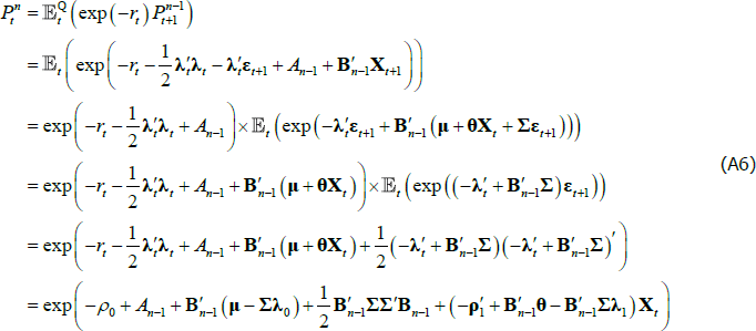
Given the above, we now show by induction that bond prices are exponentially affine in X_t. Assume that ; we will show that this implies that . Starting from Equation (A1),

where line 2 follows from Equations (A3) and (A5) and the assumption that , line 3 follows from Equation (A2), line 5 follows from the moment-generating function of a multivariate N(0,I_N) random variable, and line 6 follows from Equation (A4) and the assumed functional form of r_t. Line 6 has the desired functional form of exp, and so by equating coefficients that do and do not depend on X_t we can deduce that

To start the induction and also provide starting values for the above recursion, note that , which implies that A₀ = 0, B₀ = 0. One can also directly calculate so that A₁ = −ρ₀ and B₁ = −ρ₁.

Next consider an inflation-indexed bond that pays one unit of consumption good, or Q_{t + n}/Q_t units of nominal value, at time t + n. Here Q_t is the price level, we define inflation π_t by Q_t/Q_{t – 1} = exp(π_t), and we assume that

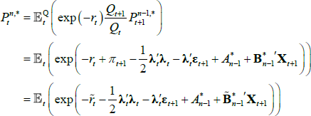
for π₀ a scalar and π₁ a vector. As with the nominal case, start by assuming that . We will show by induction that this implies that . The no-arbitrage condition for an inflation-indexed bond is given by

where, using the fact that , we define and . But, given these re-definitions, the last line now matches line 2 from the nominal bond case, so that

To provide starting values for the above recursion, note that , which implies that .

Two things are worth noting. First, in the pricing equations above, the price of risk parameters λ₀ and λ₁ are confounded with the factors describing the evolution of X_t, being μ, θ and ∑. As such, a cross-section of bond prices is not enough to fully identify the model. Second, and related to the first point, one would obtain the same pricing equations if one assumed that investors were risk neutral (so that λ₀ = 0, λ₁ = 0) and for and .