Research Discussion Paper – RDP 2021-03 Financial Conditions and Downside Risk to Economic Activity in Australia
1. Introduction
Financial stability risks are difficult to quantify and hard to map to economic outcomes. But for central banks with a financial stability mandate, the issue is crucial. For example, when inflation is contained and financial conditions are expansionary, flexible inflation-targeting central banks need to weigh the near-term benefits of easier monetary policy and stronger near-term growth prospects against the costs of doing so: specifically, the build-up of financial vulnerabilities that could pose risks to future growth and employment. The ability to quantify and communicate financial stability risks is also essential for other policymakers, such as prudential regulators and governments, who have a broader range of policy tools available to them to mitigate financial stability risks.
In addition to difficulties associated with identifying financial stability risks, policymakers face the added challenge of quantifying what the economic costs of financial instability might be. In part, this is because it is not easy to disentangle economic and financial risks that often coincide.[1] Much of the literature on this topic focuses on estimating the costs of financial crises after they have occurred. Although there is considerable variation in the way economic costs are measured, there is a broad consensus that financial crises are followed by economically significant and prolonged declines in output and output growth (see Bordo and Meissner (2016) for a comprehensive review).
It is more difficult, however, to estimate the expected costs of financial instability before any instability has been realised. Fundamentally, this requires policymakers to form an assessment of both the estimated economic cost in the event that a crisis were to occur and the estimated probability of the crisis occurring in the first place. A risk-neutral policymaker would simply multiply the expected economic cost of a crisis by the estimated probability of that crisis taking place and focus on the product of these two variables. But in practice, central banks are not risk neutral. Risk-averse policymakers will seek to reduce the probability of extremely bad outcomes occurring, and so the expected economic cost of a crisis will also be a variable of interest in its own right (Cecchetti 2006). The higher the expected cost, the more likely it is that the central bank will judge it to be optimal to sacrifice some amount of expected output so as to avoid a potentially catastrophic scenario, even if the event is not considered to be particularly likely.
While it might be tempting to rely on changes in policymakers' central forecasts to assess changes in the expected economic cost of a crisis, this is likely to be misleading in practice. This is because this approach relies on the assumption that the distribution of possible economic outcomes simply shifts higher or lower over time, without changing shape. The reality is more complex. Financial stability risks are highly nonlinear: for example, asset prices typically fall at a faster rate during post-bubble busts than they rise during the preceding booms. The global financial crisis (GFC) showed that financial stress at a single financial institution can, under certain conditions, spread quickly through the network of interbank exposures (Haldane 2009). This implies that in adverse scenarios, the distribution of economic outcomes is likely to not only shift lower, but also develop a longer left tail. This provides a strong argument for estimating expected economic costs of crises by modelling the relationship between the entire distribution of a chosen measure of financial stability and the entire distribution of economic outcomes.
The ‘growth-at-risk’ (GaR) framework was developed by Adrian, Boyarchenko and Giannone (2019) to do precisely this. The idea behind GaR is similar to ‘value-at-risk’ (VaR), which is a popular measure of risk used in finance. The concept builds on Manzan (2015) and links current financial conditions to the distribution of future economic outcomes. Specifically, it aims to quantify the magnitude of expected losses in economic activity caused by financial conditions. In practice, it achieves this by modelling the lower (left) tail of the distribution of future economic outcomes over time.
Using US data, Adrian et al (2019) show that the distribution of future GDP growth evolves over time, with the left tail (i.e. downside risk) becoming longer as prevailing financial conditions become more restrictive. The GaR approach has subsequently been applied by the Bank of Canada (Duprey and Ueberfeldt 2018), the Bank of Japan (Bank of Japan 2018), the Board of Governors of the Federal Reserve System (Kiley 2018; Loria, Matthes and Zhang 2019), the Bank of England (Aikman et al 2018) and the European Central Bank (ECB) (European Central Bank 2018). The International Monetary Fund (IMF) is also an active contributor in this area, with the GaR approach now included in its macrofinancial surveillance toolkit.
Our work contributes to this literature by developing a GaR model for Australia using a novel quantile regression approach known as ‘quantile spacings’. In addition to focusing on downside risk to aggregate GDP, we also examine other more granular indicators of macroeconomic outcomes – namely, household consumption, non-mining business investment, employment and the unemployment rate. We do this because these more granular variables have important links to financial stability in their own right. For example, excessive household debt can weigh on household consumption (Price, Beckers and La Cava 2019) and the investment of firms with excessive debt is more sensitive to interest rates (Gebauer, Setzer and Westphal 2018; Hambur and La Cava 2018). The financial conditions faced by firms can also affect their employment decisions. For example, Chodorow-Reich (2014) finds that tighter credit conditions for small businesses cause declines in employment. More generally, weak labour market outcomes could have adverse feedback effects on financial stability by creating debt-servicing challenges for some households and leading to higher rates of non-performing loans at financial institutions.
In order to implement the GaR framework for Australia we need to develop a financial conditions index (FCI) to provide a summary measure of prevailing financial conditions. Following the GFC, FCIs emerged as a potentially useful metric of financial conditions, based on the work of Hatzius et al (2010). FCIs are constructed as a weighted average of a broad range of indicators, including asset prices, credit, money, interest rates and the exchange rate. Subsequently, many policy institutions have constructed FCIs to regularly monitor financial conditions, including the IMF, a number of Federal Reserve Banks (Brave and Butters 2010), the ECB, the Bank of England (Kapetanios, Price and Young 2017) and the Bank of Canada (Gauthier, Graham and Liu 2004). One advantage of using a composite indicator such as an FCI in the GaR framework is that it is allows financial conditions to affect risk to economic activity through a variety of channels.
Similar to other economies, we find that our FCI helps to explain downside risks to future GDP growth in Australia at horizons of both one quarter and one year. We also find strong relationships between the FCI and risks to our 2 labour market indicators. However, the FCI is surprisingly of relatively little use in explaining downside risk to household consumption or business investment. While the GaR approach is a flexible and parsimonious framework, there are 2 key caveats to note.
First, it is reduced form in nature and is not well suited to identifying causal relationships. Second, there is estimation uncertainty for some of the results.
We start by describing the methodology used to implement the GaR framework in Australia, including the construction of the FCI, in the next section. Further technical details related to the FCI as well as some additional results are provided in the appendices.
2. Modelling Risks to Economic Activity from Changing Financial Conditions
We follow a four-step process to model the risks posed to economic activity from financial conditions:
- We develop a summary indicator to represent ‘financial conditions’ (the FCI), which will be an explanatory variable in subsequent regressions.
- We estimate the conditional distribution of future economic activity given current economic activity and the FCI using a novel quantile regression approach known as ‘quantile spacings’. This yields a series of fitted regressions for discrete quantiles of the distribution over time – for example, one equation for the 0.05 quantile (5th percentile) of the distribution of future economic activity, one equation for the 0.25 quantile, and so on.
- We compute a sequence of probability density functions (PDFs) by mapping the estimated discrete quantiles at each point in time to a (continuous) skewed t distribution.[2]
- We use these smoothed PDFs to quantify downside risk to future economic activity by measuring the area in the left tail of the distributions. This measure of risk is known as ‘expected shortfall’. It measures the average severity of extreme tail events given that a loss has occurred (that is, it abstracts from the probability of a loss occurring in the first place). In contrast, the more well-known VaR measure conflates the magnitude of the potential loss with the probability of it occurring.[3]
2.2 A summary indicator of financial conditions in Australia
To implement the GaR framework for Australia we require a summary indicator of financial conditions that are not otherwise directly observable. Since there is currently no existing indicator available for Australia, our first task is to develop an FCI. We follow previous work by other central banks (e.g. Brave and Butters 2010) and construct our FCI using a dynamic factor model (DFM). The model incorporates 75 individual data series covering various aspects of the financial system, including measures of: asset prices; interest rates and spreads; credit and money; debt securities outstanding; leverage; banking sector risk; financial system complexity; financial market risk; and survey measures of businesses' and consumers' views on financial conditions. Within these categories, we include a mix of Australian and US variables, with the US data included to capture spillover effects from US financial variables to other markets (Zdzienicka et al 2015). The FCI is constructed at a quarterly frequency, to match both the lowest frequency of its individual component series and the lowest frequency of the economic variables we are trying to predict.[4],[5] Appendix A.1 describes the dataset in more detail, while Appendix A.2 describes the methodology used to construct the index and Appendix A.3 sets out which components have had the most influence on the overall measure. The appropriateness of the estimation method used for the FCI is examined in Appendix A.4 and Appendix A.5 focuses on assessing the correlations between the FCI and 5 measures of economic activity, including through Granger causality tests.
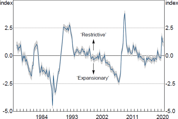
Figure 1 illustrates our estimated FCI for the time period 1976:Q4 to 2020:Q3.[6] The FCI can be interpreted as indicating that financial conditions are generally ‘restrictive’ when it takes on values greater than zero, and generally ‘expansionary’ when it takes on values less than zero.[7] The shaded region in the figure is the 95 per cent confidence interval for the FCI and its narrowness indicates that our estimate is relatively precise.[8] This high degree of precision is important as it reduces – though does not eliminate – concerns about estimation uncertainty from the use of the FCI as a ‘generated regressor’ in our subsequent quantile regressions (Bai and Ng 2006).
Note: Shaded region represents 95 per cent confidence interval
Movements in the FCI correspond to known historical events. For example, the FCI suggests financial conditions were more expansionary in the late 1980s, consistent with the rapid growth in credit and asset prices (particularly residential and commercial property prices) over that period. However, financial conditions became very restrictive around the time of the early 1990s recession as credit supply contracted sharply and commercial property prices fell from very high levels. From the mid 1990s to the early 2000s the FCI remained around zero, corresponding with the start in Australia of the period now referred to as the ‘Great Moderation’ (Simon 2001). The FCI indicates financial conditions became more expansionary from around 2006–07 before tightening significantly during the GFC (i.e. 2008–09).
More recently, financial conditions deteriorated sharply with the onset of the COVID-19 pandemic, driven in particular by declines in asset prices, weaker growth in measures of credit and money and heightened measures of financial market risk. Notably, however, our estimates suggest that financial conditions since March 2020 have not been as restrictive as they were during the GFC, similar to the results of Groen, Nattinger and Noble (2020). While this is likely due in part to the significant policy responses by central banks, fiscal authorities and financial system supervisors, it also reflects the improved resilience of the financial system since the GFC (Kearns 2020).
In addition to having a reasonably close correlation with major historical events, Granger causality tests confirm that the FCI contains predictive information about each of the 5 measures of economic activity considered in this paper (GDP, household consumption, business investment, employment and the unemployment rate). This suggests that the FCI is not simply capturing information that is already directly available from the economic variables themselves.
Having constructed an FCI with a number of appealing properties, the next step is to incorporate it into our GaR framework using the three-stage approach described below.
2.3 Stage 1: modelling the distribution of economic activity for discrete quantiles
In the first stage, we employ a variant of quantile regression (QR) to model the conditional relationship between future economic activity (the dependent variable, denoted as yt+h where h is the forecast step length) and current economic activity, current financial conditions and a constant (the explanatory variables, collectively denoted as xt). Current financial conditions are measured by the FCI.
In contrast to ordinary least squares (OLS) regressions, which estimate the conditional mean of the dependent variable, quantile regressions estimate the entire conditional distribution of the dependent variable. That is, the location, scale and shape of the distribution of the dependent variable is determined by the explanatory variables and the explanatory variables are able to have different effects on different parts of the distribution. However, one problem with using a standard QR approach when implementing the GaR framework is that it can generate quantile estimates that cross (Carriero, Clack and Marcellino 2020). This is problematic because a quantile function is, by definition, monotonic (e.g. the 0.05 quantile always lies below the 0.1 quantile), but this important property is violated if quantiles cross (e.g. the model predicted value for the 0.05 quantile lies above the prediction for the 0.1 quantile).
The crossing problem is more likely to be an issue with models that include lags of the dependent variable. This is because the set of explanatory variables that are used in estimation is determined within the model (Koenker 2005). Additionally, when crossing does occur, it is generally confined to the outlying regions of the sample space, which could affect our ability to estimate downside risk.
To avoid this potential issue, we use the ‘quantile spacing’ method proposed by Schmidt and Zhu (2016) for estimating multiple conditional quantiles. In addition to enforcing the monotonicity of the estimated quantiles, the authors show that their model can potentially better capture nonlinearities in data as well.[9] This makes the quantile spacing technique ideal for modelling GaR. It works by first modelling the level of a central quantile and then adding/subtracting a series of ‘spacing functions’ to produce the other, non-crossing, quantiles.
More formally, the quantile spacing method can be described as follows. Let be the conditional quantile function of yt+h for each quantile (0,1) such that:
Our goal is to estimate a model for p conditional quantiles associated with the quantiles and we label the jth conditional quantile of interest by Specifically, we parameterise the individual conditional quantiles as:
The process starts by modelling the level of a central quantile, which we set to be the conditional median. That is, = 0.5 for {1,...,p}. Then all other quantiles of interest are defined by adding/subtracting a series of non-negative spacing functions to this central quantile. This ensures that all quantiles will be monotonic by construction.[10]
The method we use for estimating the various coefficients follows the iterative process outlined in Schmidt and Zhu (2016). Note the interpretation of an individual coefficient within each of the spacing functions differs from a standard QR model. In this framework they represent a semi-elasticity. That is, for any , we have that:
which is the percentage change in the distance between two quantiles caused by a marginal change in xt. A positive value in a spacing below (above) the central quantile indicates that increasing xt increases downside (upside) risk by flattening the left (right) tail, all else equal.
We fit the model using quantiles = {0.05, 0.25, 0.50, 0.75, 0.95} and estimate the distribution of economic activity one quarter ahead (i.e. h = 1) for quarterly growth and 4 quarters ahead (i.e. h = 4) for year-ended growth. Besides the inclusion of the median, these are the same values originally specified by Adrian et al (2019).[11] The estimation period is 1976:Q4 to 2020:Q2, which is the minimum available sample period for our national account measures of economic activity. The main output of this process is a set of predicted values for each quantile of the distribution of economic activity over time denoted as
2.4 Stage 2: constructing a sequence of PDFs of economic activity
After fitting the quantile regression using the quantiles specified by , the next stage is to construct a sequence of continuous PDFs. We do this by mapping the fitted values from the quantile regressions onto a parametric distribution. This serves to smooth the fitted quantile regression values and provides a complete PDF. This, in turn, allows us to quantify GaR as the area in the tails of the distribution using integration. We follow Adrian et al (2019) and choose the skewed t distribution (ST).[12] The version of the ST distribution we use is the one proposed by Hansen (1994).[13] It is defined by the PDF:
where is the Gamma function, is the location of x and is the scale term. The parameter controls the skewness while q is the degrees of freedom term which controls the ‘heaviness’ of the tails (and the probability of outliers). The distribution is symmetric for = 0 and positively skewed for positive values of and vice versa.[14]
We estimate the four parameters which characterise the ST distribution for each time period in the sample. We do this by minimising the sum of squared errors between the set of fitted quantile functions and the theoretical ST distribution quantile function based on the 0.05, 0.25, 0.50, 0.75 and 0.95 quantiles as follows:
This can be viewed as an over-identified nonlinear cross-sectional regression of the predicted quantiles on the theoretical quantiles of the ST distribution.[15] With these 4 sequences of estimated parameter values we can construct a sequence of skewed t PDFs for each time period by plugging the values obtained for the 4 parameters at each time period into Equation (4).
2.5 Stage 3: quantifying tail risks to economic activity
Once we have our estimated sequences of predicted PDFs we can quantify downside and upside risks to future economic activity using expected shortfall and its counterpart, expected ‘long rise’. These two measures of risk are preferable to VaR since they summarise the tail behaviour of the estimated distribution of economic activity in absolute terms. Both measures are calculated for a given threshold quantile and are defined to be the average loss (gain) in economic activity given that a loss (gain) has occurred at or below (above) that quantile (i.e. the VaR threshold). That is, they provide a numerical answer to the question: if economic activity exceeds the quantile threshold, how bad (good) could economic outcomes be on average? In practice, this is achieved by measuring the area under the predicted PDF below (above) the relevant quantile. We can define these measures of tail risk more formally as:
Our focus will be on downside risk as measured by expected shortfall (SFt+h), but we will also highlight upside risk using expected long rise (LRt+h) to show that economic activity can respond asymmetrically to tighter and looser financial conditions.
3. How Do Financial Conditions Affect Risks to Economic Outcomes?
We repeat the processes outlined in Section 2 using 5 measures of economic activity: real GDP growth, real household consumption growth, real non-mining business investment growth, employment growth and the change in the unemployment rate. Specifically, the distributions of future growth in each measure of economic activity are estimated using current growth in the relevant measure of economic activity, the FCI and a constant as explanatory variables. For each measure of economic activity the exercise is undertaken using both quarterly and year-ended changes to examine any possible differences in the near-term and longer-term effects of financial conditions on downside risk. Future work could examine longer time horizons, creating a ‘term structure of growth at risk’ as developed in Adrian et al (2018). Alternatively, we could compile a more detailed set of explanatory variables in order to better isolate the channels through which financial conditions influence economic risk.
Our main findings are:
- The FCI contains some useful information about different parts of the distribution of each of the 5 measures of economic activity we consider. This insight would be lost if we were to focus solely on the central tendency.
- The influence of financial conditions on the different measures of future economic activity tends to be asymmetric: the lower part of the distribution is often more variable than the upper part and the estimates of downside risk are more variable than the estimates of upside risk.
- Financial conditions are estimated to be a better predictor of future downside risk to GDP and employment growth (and upside risk to the unemployment rate) than they are of household consumption and business investment.
3.1 Estimated distributions of economic activity
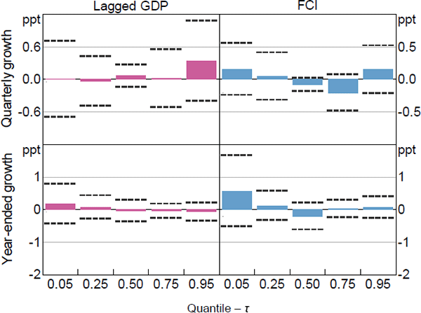
We begin by looking at the QR model results to see if the coefficient estimates related to the FCI have different values for the different quantiles examined. This will provide evidence on whether the FCI is more important for explaining some parts of the distribution of economic activity than others. Figure 2 plots the coefficient estimates (columns) and 95 per cent confidence intervals (dashed lines) for the QR with real GDP and the FCI as the independent variables for = {0.05,0.25,0.50,0.75,0.95}.[16] The top row shows the coefficient estimates for quarterly growth in GDP while the bottom row shows the coefficient estimates for year-ended growth. For space reasons we will discuss the results for all 5 measures of economic activity in this section, but choose to only present figures for GDP and employment growth. All other figures are presented in Appendix B.
We find that the coefficient point estimates take on different values for the different quantiles considered, but the differences are not statistically significant. The coefficient estimate for the FCI at the median (0.5 quantile) is negative, indicating that more restrictive financial conditions in the current period tend to result in lower median GDP growth in the future for both quarterly and year-ended horizons. However, the coefficient estimates for the FCI associated with the tails of the distribution (i.e. the 0.05 and 0.95 quantiles) are positive. This indicates that tighter current financial conditions tend to widen the distribution of future GDP growth in both the left and right tails. This widening is more pronounced for the left tail of year-ended GDP growth than it is for quarterly GDP growth. Further, most of the coefficients on the lag of GDP growth are estimated to be smaller than the coefficients on the FCI, suggesting that current financial conditions are potentially more informative than current GDP growth in explaining the quantiles of future GDP growth.
Note: Dashed lines represent 95 per cent confidence intervals computed using the stationary bootstrap proposed in Politis and Romano (1994) assuming an average block length of 8 quarters and 1,000 replications
Sources: ABS; Authors' calculations
The coefficient estimates for the other more granular measures of economic activity are broadly consistent with those for GDP growth. Generally, more restrictive current financial conditions have a negative relationship with the median future outcome for all the measures of activity (besides the unemployment rate which is, as expected, positive). However, among the other measures of economic activity, more restrictive current financial conditions only tend to widen the distribution for employment growth and the unemployment rate. In contrast, more restrictive current financial conditions tend to narrow the distribution of household consumption growth, and have a mixed effect on the upper and lower tails of the distribution of business investment (refer to Appendix B.1 for more detail).
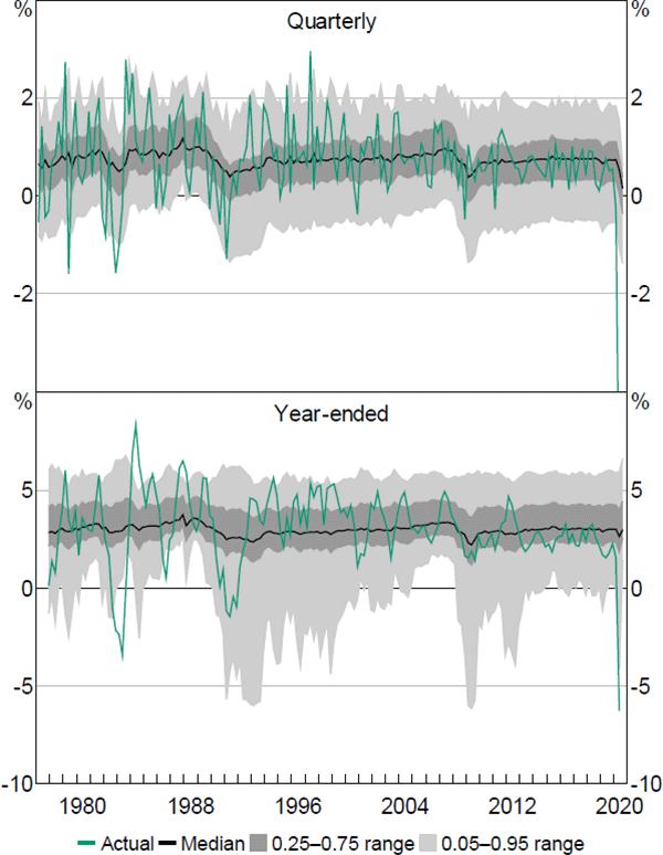
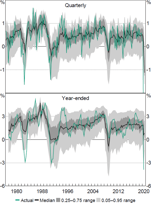
The QR coefficient estimates can now be used to compute the fitted values of the QR model. These fitted values will in turn be used to generate the sequence of continuous PDFs and estimates of downside risks to economic activity. Figures 3 and 4 display the quarterly and year-ended fitted quantiles for GDP and employment growth.
Notes: ‘GDP’ is the growth rate of real gross domestic product; actual quarterly growth rate for 2020:Q2 is –7 per cent
Sources: ABS; Authors' calculations
These figures show the estimated median, together with the estimated 0.25–0.75 and 0.05–0.95 quantile ranges for the fitted values of GDP and employment growth. The two figures highlight a key result: namely, that the outer part of the estimated distributions of both GDP and employment growth at both time horizons is more variable than the median. Further, in both cases there is also an asymmetric response. The lower parts of the estimated distributions are much more variable than the upper parts, especially for the year-ended horizon. This result is also found for the unemployment rate and, to a lesser extent, for household consumption and business investment. In the recent COVID-19 pandemic, the speed and depth of the contraction in economic activity during the March and June quarters of 2020 was far greater than that predicted by the quarterly versions of the QR model, highlighting the extreme, sudden and exogenous nature of the event. However, the year-ended estimates tended to fare much better (as the effect of June quarter 2020 is effectively ‘smoothed’), with the exception of household consumption (refer to Appendix B.2 for more detail).
Notes: ‘Employment’ is the growth rate of total employment; actual quarterly growth rate for 2020:Q2 is –5 per cent
Sources: ABS; Authors' calculations
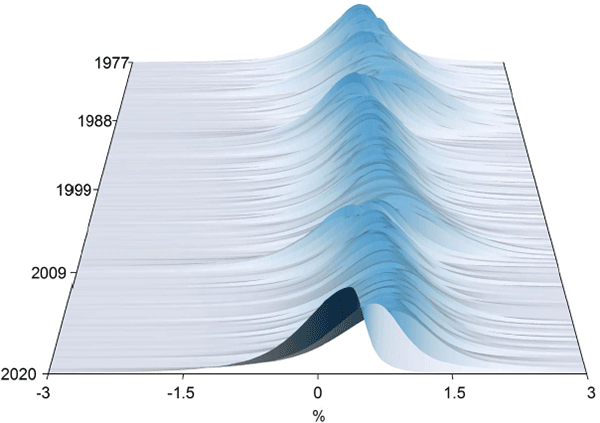
These findings underscore the benefit of modelling the entire distribution in circumstances when tail risk is of primary concern. Indeed, this result is even more evident when viewing the estimated sequences of PDFs produced from the fitted QR models for quarterly GDP growth over time (Figure 5).
Sources: ABS; Authors' calculations
The figure highlights that the location, scale and shape of the distribution for quarterly GDP growth all change over the sample period. The biggest changes occur around times of major downturns such as the 1982 recession, the 1989–91 recession, the GFC in 2008 and more recently the COVID-19 pandemic.
3.2 Downside and upside risks to economic activity
We now present the estimates of downside and upside risk to economic activity over both time horizons. These estimates are calculated as the area in the tails of the previously computed sequences of PDFs. In computing these measures of risk we employ a threshold quantile of = 0.05 for both horizons. The results for GDP growth and employment growth are displayed in Figures 6 and 7.
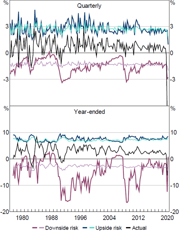
Notes: ‘GDP’ is the growth rate of real gross domestic product; actual quarterly growth rate for 2020:Q2 is –7 per cent; is set equal to 5 per cent; thicker darker-coloured line is estimated with the FCI; thinner lighter-coloured line is estimated without the FCI
Sources: ABS; Authors' calculations
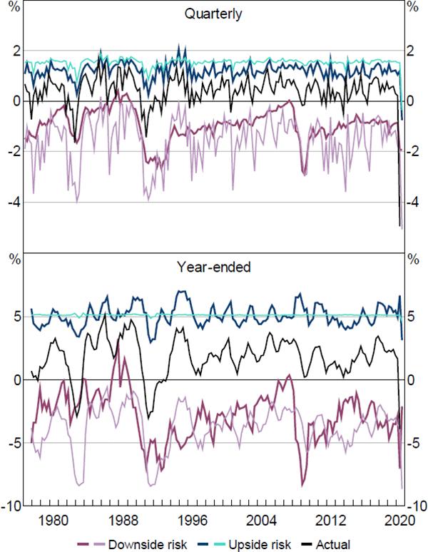
Notes: ‘Employment’ is the growth rate of total employment; is set equal to 5 per cent; thicker darker-coloured line is estimated with the FCI; thinner lighter-coloured line is estimated without the FCI
Sources: ABS; Authors' calculations
The ‘Downside risk’ lines show our estimate of what realised growth in either GDP or employment would have been if it was in the bottom 5 per cent of the fitted distributions at each point in time.[17] Similarly, the ‘Upside risk’ lines show our estimate of what growth in GDP or employment would have been if it was in the top 5 per cent of the fitted distributions at each point in time. The ‘Actual’ line represents the observed values for GDP growth and employment growth. For both downside and upside risk, the thicker darker-coloured lines signify the estimates obtained when both economic activity and financial conditions are included as explanatory variables in the QR model. In contrast, the thinner lighter-coloured lines signify the equivalent estimates when the FCI is excluded from the QR model and only current economic activity is used in estimation. As such, the difference between the thicker and thinner lines in each figure demonstrates the contribution that financial conditions make to the estimate of tail risk for that measure of economic activity.
The results show that estimates of downside and upside risk for GDP growth are much more variable when financial conditions are accounted for; especially around 1991–92 and 2008–09. This was also the case in the first half of 2020, with the model's estimates of downside risk to GDP growth performing relatively better in capturing the actual decline in GDP growth (at both horizons) than the estimates that exclude financial conditions as an explanatory variable. This suggests that the FCI contains useful information about downside risks to GDP growth, over and above measures of current GDP growth. For employment growth, however, the results indicate the FCI is more useful for explaining downside risks at a year-ended horizon than at a quarterly horizon.
The FCI also makes meaningful contributions to the estimates of upside risk to the unemployment rate (i.e. the risk of a large increase in unemployment), predominately at a year-ended time horizon. Downside risk is estimated to be more variable than upside risk for GDP and employment, while upside risk to the unemployment rate is estimated to be more variable than downside risk. In contrast, the aggregate FCI seems to make relatively little difference to the estimates of downside risk for household consumption and business investment, with the results for business investment also puzzling in that they display more variation in upside risk than they do in downside risk (refer to Appendix B.3 for detailed results for these activity measures). It is possible that more disaggregated measures of financial conditions could yield different results.
Overall, the results indicate that the ability of financial conditions to explain changes in downside risk to different measures of economic activity in Australia is mixed. For some series, financial conditions seem to provide useful additional information (i.e. GDP, employment and the unemployment rate) while for other series, financial conditions seem less informative (i.e. household consumption and business investment). It is possible that a model with more structure would allow us to more clearly identify the link between financial conditions and macroeconomic risk – including for variables like household consumption and business investment – however, this is beyond the scope of the GaR framework presented in this paper. Moreover, it is also important to note that because financial crises in Australia have been rare (in the period covered by our dataset there have only been two significant financial crises) the FCI's ability to contribute additional information about tail risk is likely to be limited to these two time periods.
4. Conclusion
We make 3 important contributions. First, we develop a financial conditions index for Australia. This measure incorporates a broad range of individual indicators over a relatively long time period. Our measure correlates closely with previous financial boom and bust cycles in Australia, and also appears to have some ability to predict some measures of economic activity. In light of this, we suggest the FCI is a useful complement to existing qualitative and disaggregated approaches to monitoring financial conditions and financial stability risks in Australia.
Second, we use this FCI to develop a growth-at-risk framework for Australia. This adds to a rapidly growing body of literature which has developed similar models for a range of other countries. The GaR approach allows us to quantify the effect of current financial conditions on expected future downside risks to economic activity. We find that downside risk to economic activity from changes in financial conditions tends to be more volatile than upside risk. This insight would be missed if we only considered the central tendency and not the full distribution of economic outcomes as they relate to financial conditions. As such, the approach provides a potential way of quantifying the economic costs of financial instability risks.
Third, in contrast to other papers which have focused solely on quantifying downside risk to GDP growth, we examine the relationship between financial conditions and a broader range of macroeconomic variables. In particular, we expand the GaR framework to also examine household consumption, business investment and labour market variables (both employment growth and the unemployment rate). All of these variables have potentially important links to financial stability in their own right. We find that our FCI provides information about downside risks to GDP and employment growth and upside risks to changes in the unemployment rate. However, the FCI is much less useful for explaining downside risks to growth in household consumption and business investment.
Finally, we note that there are some limitations of the GaR approach. First, while the GaR framework is a flexible and parsimonious approach, it is also a reduced-form model and most appropriate for comparative statics analysis. To get a better understanding of the links between financial conditions and economic activity would require a more structured modelling approach. Second, there is some uncertainty with some of our estimation results. As such, the GaR approach is best thought of as a useful complement to other existing approaches to monitoring the potential economic costs of financial instability, rather than a tool to be relied on in isolation.
Appendix A: Estimating a Financial Conditions Index for Australia
A.1 The financial conditions index dataset
The specific series used to estimate the FCI were chosen to cover a broad range of indicators of financial conditions. The rationale is that financial instability can manifest itself, and impact on the real economy, in a wide variety of ways. This means it is not only important to include variables that have historically shown themselves to be relevant (e.g. housing and commercial property prices) but also to include variables that are emerging as potential sources of future risk (e.g. indicators of financial system complexity). The set of variables used in this paper have considerable, though not complete, overlap with those that have been identified as important in other research (e.g. Aikman et al 2018; Prasad et al 2019).
Our main selection criterion was that the series needed to be available at least since the mid 1990s so as to capture as much time variation as possible, particularly given that historical episodes of financial instability in Australia have so far been few and far between.[18] One downside of this approach is that it excludes some measures that are likely to be very relevant today – and going forward – because they do not have sufficiently long histories. Relatedly, the approach is vulnerable to the criticism that it can over-weight measures that happen to be available for longer periods of time.
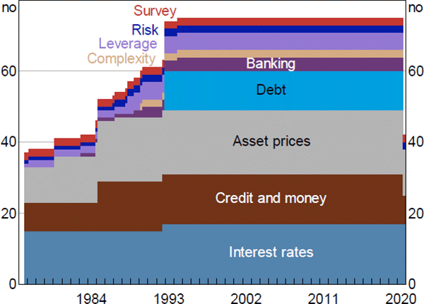
The resulting set of variables we use can be grouped into the following categories: asset prices (18 series); interest rates and spreads (17); credit and money (14); debt securities outstanding (11); indicators of leverage (5); indicators of banking sector risk (4); indicators of financial system ‘complexity’ (2); indicators of financial market risk (2); and surveys' indicators of businesses' and consumers' views on financial conditions (2). Our dataset spans the sample period 1976:Q3 to 2020:Q3, however, many financial variables we use only have a relatively short history which means our dataset is unbalanced. It starts with 37 series, increases to 54 series by 1987 and to the full dataset of 75 series by mid 1994 but, due to data availability, there are only 42 series for September quarter 2020 (Figure A1).
Sources: ABS; ACCI–Westpac; APRA; ASX; Austraclear Limited; Australian Office of Financial Management; Authors' calculations; Bloomberg; CoreLogic; Federal Reserve Bank of St. Louis; MSCI; Private Placement Monitor; RBA; Refinitiv; State borrowing authorities; Westpac and Melbourne Institute
Before estimating the FCI we transform all variables in our dataset to be stationary and standardise them to have zero mean and unit variance.[19] Because all of our variables are nominal, we control for potential structural breaks in the mean of each series in our dataset following the introduction of inflation targeting by the RBA in 1993 by ‘dynamically demeaning’ each series using a rolling 10-year backward-looking estimate of the sample mean (rather than using the full sample mean). Using a rolling estimate of the sample mean allows us to be agnostic about the precise date the break occurred and is preferable to estimating a specific break date for each series in the dataset, which could be subject to large estimation uncertainty.[20] The choice of a 10-year window follows Kamber, Morley and Wong (2018), but is not specifically related to the length of business or financial cycles in our case. Note, dynamically demeaning all series even if no series has a structural break in the mean should not cause any estimation problems. If there is no structural break in a particular series then the rolling window estimated sample mean for that series should be equal to its full sample mean.
Some previous papers have ‘purged’ the financial data of correlations with measures of economic activity before estimating the FCI by using the residuals from regressions of the financial variables on a set of variables related to ‘macroeconomic conditions’ (e.g. Hatzius et al 2010). However, we follow Kapetanios et al (2017) who argue that purging the data with a prior regression may reduce its usefulness as a summary measure. For example, if the only common shock in the economy at a given point in time was financial in nature, then this type of analysis would amount to purging the financial series of precisely the information we are aiming to summarise. Table A1 provides a complete list of all series we use to estimate the FCI and specifies the source, the start and end dates as well as the specific transformation we apply to each series.
| No | Variable | Source | Economy | Start date | End date | Transformation code |
|---|---|---|---|---|---|---|
| Survey measures | ||||||
| 1 | Business: difficulty getting finance | ACCI-WBC | Aus | 1966:Q2 | 2020:Q3 | FD |
| 2 | Consumer: family finances now | WBC-MI | Aus | 1974:Q4 | 2020:Q3 | LV |
| Interest rates and spreads | ||||||
| 3 | Overnight cash rate (OCR) | RBA | Aus | 1976:Q3 | 2020:Q3 | FD |
| 4 | 3-month bank bill rate | ASX; RBA | Aus | 1976:Q3 | 2020:Q3 | FD |
| 5 | 3-year Australian Government security (AGS) yield | RBA | Aus | 1992:Q3 | 2020:Q3 | FD |
| 6 | 5-year AGS yield | RBA | Aus | 1976:Q3 | 2020:Q3 | FD |
| 7 | 10-year AGS yield | RBA | Aus | 1969:Q3 | 2020:Q3 | FD |
| 8 | Spread: 3-month bank bill to OCR | ASX; RBA | Aus | 1972:Q1 | 2020:Q3 | LV |
| 9 | Spread: 3-year AGS to OCR | RBA | Aus | 1992:Q3 | 2020:Q3 | LV |
| 10 | Spread: 5-year AGS to OCR | RBA | Aus | 1969:Q3 | 2020:Q3 | LV |
| 11 | Spread: 10-year AGS to OCR | RBA | Aus | 1976:Q3 | 2020:Q3 | LV |
| 12 | Federal funds rate (FFR) | FRED | US | 1959:Q3 | 2020:Q3 | FD |
| 13 | 3-month Treasury bill (Tbill) yield | FRED | US | 1959:Q3 | 2020:Q3 | FD |
| 14 | 3-year Treasury bond (TB) yield | FRED | US | 1959:Q3 | 2020:Q3 | FD |
| 15 | 10-year TB yield | FRED | US | 1959:Q3 | 2020:Q3 | FD |
| 16 | Spread: 3-month Tbill to FFR | FRED | US | 1959:Q3 | 2020:Q3 | LV |
| 17 | Spread: 3-year TB to FFR | FRED | US | 1959:Q3 | 2020:Q3 | LV |
| 18 | Spread: 10-year TB to FFR | FRED | US | 1959:Q3 | 2020:Q3 | LV |
| 19 | Spread: 10-year AGS to 10-year USTB | RBA; FRED | Aus/US | 1969:Q3 | 2020:Q3 | LV |
| Credit and money | ||||||
| 20 | Total credit | RBA | Aus | 1976:Q3 | 2020:Q3 | LD |
| 21 | Housing credit | RBA | Aus | 1976:Q3 | 2020:Q3 | LD |
| 22 | Personal credit | RBA | Aus | 1976:Q3 | 2020:Q3 | LD |
| 23 | Business credit | RBA | Aus | 1976:Q3 | 2020:Q3 | LD |
| 24 | Owner-occupier housing loan approvals (excl refinancing) | ABS | Aus | 1985:Q1 | 2020:Q2 | LD |
| 25 | Investor housing loan approvals (excl refinancing) | ABS | Aus | 1985:Q1 | 2020:Q2 | LD |
| 26 | Commercial fixed term loan approvals (excl refinancing) | ABS | Aus | 1985:Q1 | 2020:Q2 | LD |
| 27 | Commercial revolving credit approvals (excl refinancing) | ABS | Aus | 1985:Q1 | 2020:Q2 | LD |
| 28 | Personal fixed term loan approvals (excl refinancing) | ABS | Aus | 1985:Q1 | 2020:Q2 | LD |
| 29 | Personal revolving credit approvals (excl refinancing) | ABS | Aus | 1985:Q1 | 2020:Q2 | LD |
| 30 | M1 | RBA | Aus | 1975:Q1 | 2020:Q3 | LD |
| 31 | M3 | RBA | Aus | 1976:Q3 | 2020:Q3 | LD |
| 32 | Broad money | RBA | Aus | 1976:Q3 | 2020:Q3 | LD |
| 33 | Money base | RBA | Aus | 1975:Q1 | 2020:Q3 | LD |
| Asset prices | ||||||
| 34 | Dwelling price index | CoreLogic | Aus | 1980:Q1 | 2020:Q3 | LD |
| 35 | House price index | CoreLogic | Aus | 1980:Q1 | 2020:Q3 | LD |
| 36 | Apartment price index | CoreLogic | Aus | 1980:Q1 | 2020:Q3 | LD |
| 37 | Dwelling price index | FRED | US | 1987:Q1 | 2020:Q2 | LD |
| 38 | All commercial property return index | MSCI | Aus | 1984:Q4 | 2020:Q2 | LD |
| 39 | Retail property return index | MSCI | Aus | 1984:Q4 | 2020:Q2 | LD |
| 40 | Office property return index | MSCI | Aus | 1984:Q4 | 2020:Q2 | LD |
| 41 | Industrial property return index | MSCI | Aus | 1984:Q4 | 2020:Q2 | LD |
| 42 | ASX 200 Index | Refinitiv | Aus | 1973:Q1 | 2020:Q3 | LD |
| 43 | ASX 200 Financials Index | Refinitiv | Aus | 1973:Q1 | 2020:Q3 | LD |
| 44 | ASX 200 Real Estate Index | Refinitiv | Aus | 1973:Q1 | 2020:Q3 | LD |
| 45 | ASX 200 Resources Index | Refinitiv | Aus | 1973:Q1 | 2020:Q3 | LD |
| 46 | ASX 200 Industrials Index | Refinitiv | Aus | 1973:Q1 | 2020:Q3 | LD |
| 47 | S&P 500 Index | FRED | US | 1960:Q1 | 2020:Q3 | LD |
| 48 | RBA Index of Commodity Prices (AUD) | RBA | Aus | 1959:Q3 | 2020:Q3 | LD |
| 49 | Gold (3pm London bullion market, USD) | FRED | US | 1968:Q2 | 2020:Q3 | LD |
| 50 | Crude oil (West Texas intermediate, USD) | FRED | US | 1968:Q2 | 2020:Q3 | LD |
| 51 | Australian dollar trade-weighted index | RBA | Aus | 1970:Q3 | 2020:Q3 | LD |
| Debt securities outstanding | ||||||
| 52 | Short-term: Australia: banks | APRA; Austraclear Limited; RBA | Aus | 1992:Q4 | 2020:Q2 | LD |
| 53 | Short-term: Australia: non-financial corporations | Austraclear Limited; RBA | Aus | 1992:Q4 | 2020:Q2 | LD |
| 54 | Long-term: banks | Bloomberg; RBA | Aus | 1992:Q4 | 2020:Q2 | LD |
| 55 | Long-term: Australia: non-financial corporations | Bloomberg; RBA | Aus | 1992:Q4 | 2020:Q2 | LD |
| 56 | Short-term: Australia: government | AOFM; Austraclear Limited; RBA | Aus | 1992:Q4 | 2020:Q2 | LD |
| 57 | Long-term: Australia: government | AOFM; RBA; State borrowing authorities | Aus | 1992:Q4 | 2020:Q2 | LD |
| 58 | Long-term: overseas: non-government | ABS; Bloomberg; Private Placement Monitor; RBA | Aus | 1992:Q4 | 2020:Q2 | LD |
| 59 | Short-term: Australia: asset-backed securities | ABS; Bloomberg; RBA | Aus | 1992:Q4 | 2020:Q2 | LD |
| 60 | Long-term: Australia: asset-backed securities | ABS; Bloomberg; RBA | Aus | 1992:Q4 | 2020:Q2 | LD |
| 61 | Long-term: overseas: asset-backed securities | ABS; Bloomberg; RBA | Aus | 1992:Q4 | 2020:Q2 | LD |
| 62 | Residential mortgage-backed securities | ABS; Bloomberg; RBA | Aus | 1992:Q4 | 2020:Q2 | LD |
| Banking sector | ||||||
| 63 | Tier 1 capital ratio | APRA; RBA | Aus | 1989:Q2 | 2020:Q2 | FD |
| 64 | Non-performing assets ratio | APRA; RBA | Aus | 1990:Q2 | 2020:Q2 | FD |
| 65 | Distance to default | RBA | Aus | 1983:Q1 | 2020:Q2 | LV |
| 66 | Wholesale debt spread to AGS | Bloomberg; RBA | Aus | 1994:Q2 | 2020:Q2 | FD |
| Financial system complexity (ratio) | ||||||
| 67 | Total financial institutions' assets to nominal GDP | ABS; RBA | Aus | 1990:Q1 | 2020:Q2 | LD |
| 68 | Total off-balance sheet business to total fixed income assets | ABS; RBA | Aus | 1990:Q1 | 2020:Q2 | LD |
| Leverage measures (ratio) | ||||||
| 69 | Household debt to assets | ABS; RBA | Aus | 1988:Q3 | 2020:Q2 | LD |
| 70 | Household debt to income | ABS; RBA | Aus | 1988:Q2 | 2020:Q2 | LD |
| 71 | Household interest payments to income | RBA | Aus | 1977:Q1 | 2020:Q2 | LD |
| 72 | Current account balance to nominal GDP | ABS | Aus | 1959:Q3 | 2020:Q2 | FD |
| 73 | Net total foreign liabilities to nominal GDP | ABS | Aus | 1988:Q3 | 2020:Q2 | FD |
| Risk indicators | ||||||
| 74 | Chicago Board Options Exchange equity volatility | FRED | US | 1986:Q4 | 2020:Q3 | LV |
| 75 | Moody's corporate bond yield spread: BAA to AAA | FRED | US | 1959:Q3 | 2020:Q3 | LV |
| Notes: ‘ABS’ is Australian Bureau of Statistics, ‘ACCI-WBC’ is Australian Chamber of Commerce and Industry–Westpac, ‘AOFM’ is the Australian Office of Financial Management, ‘FRED’ is Federal Reserve Economic Database, Federal Reserve Bank of St. Louis, ‘WBC-MI’ is Westpac and Melbourne Institute; ‘Transformation code’ indicates the method used to transform the data to be stationary if necessary, ‘FD’ indicates first difference, ‘LD’ indicates log difference and ‘LV’ indicates level | ||||||
A.2 Constructing the financial conditions index
The general form of the DFM we use to estimate the FCI follows Bai and Wang (2015) and is defined as:
where yt is N × 1 vector of observables, ft is a q × 1 vector of the dynamic factors, and is the dynamic factor loadings for ft – j with j = 0,1,...,s and t = 1,...,T. The dynamic factors follow a VAR(p) process with a q × q matrix of autoregressive coefficients (with all roots outside the unit circle). The number of dynamic factors is q (the dimension of ft) which is irrespective of s and p.
The covariance matrix of in the measurement equation is given by R with dimension N × N and is restricted to be a diagonal matrix. In the state equation, the covariance matrix of corresponds to the q × q matrix Q. We assume that (i.e. the 2 noise processes are independent). This specification of the DFM has 2 different sources of dynamics. First, there are s lagged factors representing a dynamic relationship between the observable series yt and the factors ft. Second, the dynamics of the factors is assumed to be captured by a VAR(p) process. Bai and Wang (2015) argue that it is the first source of dynamics that makes this specification a true dynamic factor model because it is these dynamics that make the biggest distinction between dynamic and static factor analysis.[21] The state-space representation of the DFM specified by Equation (A2) is:
The measurement equation takes the form of a static factor model (Stock and Watson 2002) with r = q (s + 1) static factors. Now, define k = max(p,s + 1) and set if k = s + 1 > p.
Let , then the N × qk factor loadings matrix the qk × qk matrix of VAR coefficients and the qk × q selector matrix G have the following form:
when k = p > s, let be a subvector of Ft. Then the factor loadings matrix and the VAR coefficient matrix become:
Note, the selector matrix G does not change in this alternative setting. The benefit of this modelling strategy over others, such as traditional static factor models based on principal components analysis (PCA), is that it explicitly incorporates dynamics into the estimation and can easily and efficiently handle unbalanced datasets such as the one we use.
When implementing the DFM we assume one common factor (i.e. q = 1) is adequate to capture the common variation we are most interested in from our dataset. This decision was made because we want a single index to represent ‘financial conditions’. Multiple factors would require us to combine them into a single index and it is unclear what the optimal way to do this is. Moreover, the modified Bai and Ng (2002) information criterion proposed by Coroneo, Giannone and Modugno (2016) suggests one factor is sufficient.[22]
The dynamics of the factor are assumed to follow an AR(1) process (i.e. p = 1). This was determined by the Schwarz information criterion (SIC), together with plots of the sample autocorrelation function (ACF) and sample partial ACF for the common factor based on an initial estimate of the common factor obtained by PCA.
We choose to include one lag of the factor in the measurement equation (i.e. s = 1) because some of the series in our dataset are market determined. These series will tend to be less persistent (and potentially more volatile) than the other series in our dataset which are not market determined. A DFM with dynamic loadings will be able to accommodate this explicitly.
Following Doz, Giannone and Reichlin (2011, 2012) we estimate the DFM by quasi-maximum likelihood.[23] Estimation consists of 2 parts. First, the parameters of the state-space representation of the DFM are obtained by applying PCA to a balanced subset of the dataset which contains all 75 series. Second, the Kalman filter is applied on the original unbalanced dataset in order to obtain estimates of the factors using only the information available at each point in time.
For the observations Y = {y1,...,yT}, factors F = {F1,...,FT} and parameter vector the complete data log likelihood is given by:
We estimate the parameter vector using the expectation-maximisation (EM) algorithm and the Kalman filter and Rauch-Tung-Striebel (RTS) smoother recursions (for more details, see Anderson and Moore (1979)). To do this, we set the initial values in the state-space equations using the first r principal components-based estimates of the factors and OLS estimates of the parameters and Q treating the principal components factors as the true common factors. From these starting values we then alternate between 2 steps. First, we estimate the expected value of the common factors given the data and previously estimated model parameters (the ‘E-step’). This involves running the Kalman filter and RTS smoother recursions and getting a new estimate of the common factors denoted by where is the vector of estimated model parameters from the previous step. Then using these updated estimates of the common factors we compute new parameter estimates by maximising the expected log likelihood with respect to (the ‘M-step’).
To account for missing observations in yt we define the known matrix Wt which is a diagonal matrix of size N with the ith diagonal element equal to zero if yi,t is missing and equal to one otherwise. The matrix Wt acts a selector matrix and ensures only the available data are used in the Kalman filter and RTS smoother recursions. The updating equations for the parameters and Q are as follows:
To compute the next we use:
To compute the next we use:
To compute the next R we use:
To compute the next Q we use:
The initial state F0 and initial state variance P0 are given by:
See Ghahramani and Hinton (1996) and Bańbura and Modugno (2014) for more details on these calculations. We judge convergence to be when cm is less than 10–4, with cm given by:
and m = 1,...,M is the number of evaluations needed to achieve convergence up to a maximum M set by the researcher. We set M = 500 but we only needed 8 evaluations in our case.
A convenient feature of this specification is that the computational complexity of the Kalman filter and RTS smoother recursions depends only on the size of the state. In our case this corresponds to r and is independent of the size of the cross-section N. Note, while the EM algorithm will converge to a maximum, it is not guaranteed to find the global maximum and can converge to a local maximum. We can reduce the probability of this occurring by starting the algorithm with the PC-based estimates which are consistent for large cross-sections (see Stock and Watson (2002) and Bai and Ng (2002)).
A common issue with estimating factor models is the lack of identification. In our case this means the likelihood of our model is invariant to any invertible linear transformation of the factors. That is, for any invertible matrix H the parameters = and are observationally equivalent and hence is not identifiable from the data. In order to achieve identifiability of , we need to impose an identifying restriction. We implement the restriction ‘DFM2’ suggested by Bai and Wang (2015).[24] This identifying restriction specifies the first q × q block of in to be an identity matrix:
where is an (N – q) × q unrestricted block of . This parameterisation of is also called the ‘named factor’ normalisation because it associates each factor with a specific variable (Stock and Watson 2016).
When implementing this identifying restriction it is important to order the variables in Y so that the first q variables are the naming variables. In practice, the naming variables need to be reasonably different from each other and sufficiently representative of groups of other variables so that the innovations to their common components span the same space as the factor innovations. In our work we choose to put the series ‘survey: difficulty getting finance for business’ as the first series. Increases in this series reflect greater difficulty for businesses getting access to finance while decreases in this series reflect less difficulty for businesses in getting access to finance. A benefit of this normalisation is that it also identifies the sign of the estimated common factor. It is common for more restrictive financial conditions to be reflected by increases in the FCI and for more expansionary financial conditions to be reflected by decreases in the FCI (see Brave and Butters (2010)). Hence, being able to impose this sign convention with our FCI is beneficial. The named factor normalisation means the interpretation of the factor loadings on the other variables changes. They become measures of the correlation of each series with the factor relative to the named factor series.
To impose this identifying linear restriction in estimation we need to modify the M-step used to estimate to incorporate the linear restriction specified by:
where is a selector matrix with dimension q2 × (N × r) with 0 or 1 elements specifying the coefficients that will be restricted. The vector is of dimension q2 × 1 also with 0 or 1 elements and are the values that the coefficients will be restricted to be. The updating equation incorporating the identifying restriction for becomes:
where is the estimated factor loadings with the identifying restriction and is the unrestricted estimated factor loadings given previously by Equation (A6), see Wu, Pai and Hosking (1996) and Bańbura and Modugno (2014) for more information.
A.3 Which series are most important for financial conditions?
The sign and magnitude of the combined values of the 2 factor loadings for each series indicate the relative strength and direction of that series' relationship with the estimated FCI. Figure A2 highlights the 10 most important series by positive and negative combined weights. Series with a negative (positive) combined weight tend to move in the opposite (same) direction to the FCI, falling (rising) when the FCI indicates financial conditions are restrictive and rising (falling) when the FCI indicates financial conditions are expansionary.
The series which are most strongly related to the contemporaneous value of the FCI tend to have negative weights. These same series also tend to be negatively related to the one-period lag of the FCI as well. These include property prices, growth in credit aggregates and one survey measure related to consumer expectations of their finances. Of these, commercial property has the highest combined weighting and as a result has the strongest relationship with the FCI. This is unsurprising given the highly procyclical nature of commercial property returns during the only 2 episodes of significant financial instability in our sample. Coupled with the fact that the commercial property sector has historically been a relatively important source of risk to banks' balance sheets (Ellis and Naughtin 2010), these results underscore the importance of monitoring developments in this sector on an ongoing basis.
In contrast, only one-quarter of the dataset are positively related to the FCI, with the magnitude of the combined weights typically much smaller than those series with negative signs. The strongest positive correlations belong mostly to interest rate spreads. Note, we have not included the series ‘survey: difficulty getting finance for business’ since the first factor loading is restricted to be unity by design (see Appendix A.2).
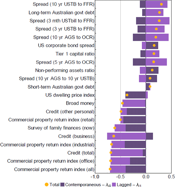
Note: Weights are the estimated factor loadings for each series excluding the named factor series ‘survey: difficulty getting finance for business’
Sources: ACCI–Westpac; APRA; Austraclear Limited; Australian Office of Financial Management; Authors' calculations; CoreLogic; Federal Reserve Bank of St. Louis; MSCI; RBA; State borrowing authorities; Westpac and Melbourne Institute
A.4 Robustness checks for the FCI
We undertake 2 checks of our preferred estimated FCI to confirm its soundness as a measure of financial conditions. The first is a comparison of the DFM methodology against an alternative method for estimating the FCI. The second is a comparison of our preferred estimated FCI (estimated using the DFM approach) and the named factor series ‘survey: difficulty getting finance for business’. The named factor series is the one we choose to restrict the factor loading to be unity in estimation for identification purposes. Both comparisons are shown in Figure A3.
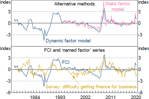
Notes: The ‘Static factor model’ estimates were renormalised to match the profile of the dynamic factor model FCI; the ‘named factor’ series has been standardised to have zero mean and unit variance
The top panel compares our preferred estimated FCI with another FCI produced using a static factor model (SFM). The DFM technique is preferable to the SFM technique since it allows the FCI to be estimated over a longer time period (SFMs are estimated by PCA and require balanced datasets). Further, since the DFM explicitly incorporates dynamics, it produces an indicator that appears smoother than the indicator based on the SFM estimate.
The bottom panel shows the estimated FCI and the named factor series ‘survey: difficulty getting finance for business’. Both series display a reasonably similar ‘low frequency’ pattern, but the movements between the two series are not exactly the same. This shows that the named factor series is not significantly influencing the profile of the estimated FCI besides helping to identify its scale, as intended.
A further robustness check of the DFM methodology is to formally test whether the dataset as a whole supports the inclusion of a lag of the factor in the measurement equation. We test this using a likelihood ratio ( LR ) test.[25] This is easy to do since we get the log likelihood as a by-product of the Kalman filter. To compute the LR statistic we estimate the DFM twice. Once with the lag included to get the value of the unrestricted log likelihood and again with the lag excluded to get the value of the restricted log likelihood The LR test statistic is then computed as:
where k is the number of restrictions to be tested. Under the null hypothesis the test is distributed as chi-squared with k degrees of freedom. The test result is shown in Table A2. The test statistic is very large at 1,091 and with k = 75 parameter restrictions the associated p-value is effectively zero.
This suggests there is little evidence against the DFM methodology we have used to construct the FCI.
| Number of parameter restrictions ( k ) | 75 |
|---|---|
| Unrestricted log likelihood ( ) | −16,145.5 |
| Restricted log likelihood ( ) | −16,691.2 |
| Test statistic | 1,091.4 |
| p-value | 0.0 |
| Note: Test statistic is computed as −2 which is distributed as chi-squared with k degrees of freedom under the null | |
A.5 Assessing the relationship between financial conditions and economic outcomes
We start by assessing the FCI's ability to predict 5 separate summary measures of economic activity: real GDP, real household final consumption expenditure, the unemployment rate, employment and real non-mining business investment. We examine both quarterly and year-ended changes in these variables over the period 1976:Q4 to 2020:Q2.[26]
Figure A4 plots the FCI against the 5 measures of economic activity for quarterly and year-ended time horizons. Each series has been standardised to have zero mean and unit variance. Most series exhibit reasonable contemporaneous relationships with the FCI, although the strength varies. Four of the measures of economic activity are negatively related to financial conditions (more restrictive financial conditions correspond to weaker growth), while change in unemployment rate has a positive relationship (more restrictive financial conditions are associated with an increase in the unemployment rate).
Estimates of the sample cross-correlation between the measures of activity and the FCI for both time horizons are provided in Table A3.
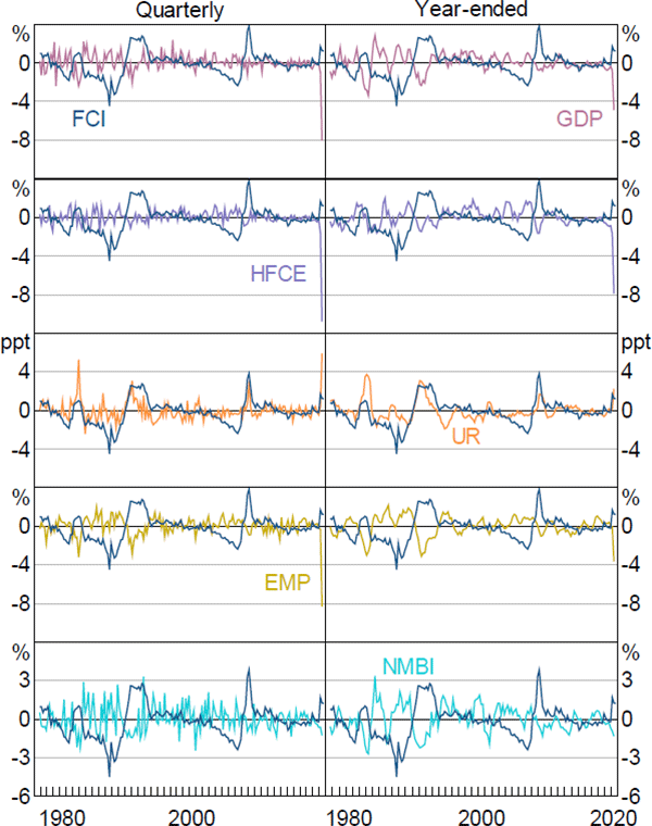
Notes: All economic activity series are standardised to have zero mean and unit variance; ‘GDP’ is the growth rate of real gross domestic product; ‘HFCE’ is the growth rate of real household final consumption expenditure; ‘UR’ is the change in the total unemployment rate; ‘EMP’ is the growth rate of total employment; ‘NMBI’ is the growth rate of real business investment excluding mining investment
Sources: ABS; Authors' calculations; RBA
The contemporaneous sample correlations between the measures of economic activity and the FCI are strongest for the 2 labour market variables and weakest for consumption. Across variables, correlations tend to be stronger for year-ended, rather than quarterly, changes reflecting the fact that year-ended changes are relatively smoother. The sample cross-correlation between these measures of economic activity and the FCI at different lag lengths suggest there might be a lead/lag relationship between the FCI and the various measures of economic activity.
| Quarterly | Year-ended | ||||||
|---|---|---|---|---|---|---|---|
| Contemporaneous | Maximum(a) | Lag(b) | Contemporaneous | Maximum(a) | Lag(b) | ||
| GDP | −0.27 | −0.27 | 0 | −0.43 | −0.45 | 1 | |
| Consumption | −0.21 | −0.22 | 1 | −0.30 | −0.35 | 1 | |
| Unemployment rate | 0.44 | 0.44 | 0 | 0.51 | 0.55 | 1 | |
| Employment | −0.46 | −0.47 | 1 | −0.60 | −0.67 | 1 | |
| Business investment | −0.28 | −0.28 | −1 | −0.46 | −0.46 | 0 | |
|
Notes: All series are in growth rates besides the unemployment rate which is in differences
|
|||||||
However, sample cross-correlations between two serially correlated time series can sometimes indicate spurious relationships (see Cryer and Chan (2008)). To formally assess these potential lead/lag relationships we use Granger causality tests. This attempts to determine if the lags of one time series have information that is useful for predicting another time series over and above the information already contained in the lags of that second series. The test can be sensitive to the choice of lag length, so we test for lag lengths from one to four quarters.[27] We can infer Granger causality when there is evidence that the FCI Granger-causes the measure of economic activity and no evidence that the measure of economic activity Granger-causes the FCI. The results are in Table A4.
The results suggest that the FCI does contain predictive information about the 5 measures of economic activity at a quarterly time horizon, although the results for household consumption are only significant at the 10 per cent level for the first lag. At a year-ended time horizon the results are similar for GDP, household consumption, the unemployment rate and employment. In contrast, the FCI only provides additional predictive information for business investment at longer lag lengths (i.e. lags greater than 2).
| Lag length | ||||
|---|---|---|---|---|
| 1 | 2 | 3 | 4 | |
| Quarterly | ||||
| GDP does not Granger-cause FCI | 0.85 | 1.00 | 1.00 | 1.00 |
| FCI does not Granger-cause GDP | 0.02 | 0.00 | 0.00 | 0.00 |
| HFCE does not Granger-cause FCI | 1.00 | 1.00 | 1.00 | 1.00 |
| FCI does not Granger-cause HFCE | 0.09 | 0.00 | 0.01 | 0.01 |
| UR does not Granger-cause FCI | 1.00 | 1.00 | 1.00 | 1.00 |
| FCI does not Granger-cause UR | 0.00 | 0.00 | 0.00 | 0.00 |
| EMP does not Granger-cause FCI | 0.74 | 0.23 | 0.26 | 0.74 |
| FCI does not Granger-cause EMP | 0.00 | 0.00 | 0.00 | 0.00 |
| NMBI does not Granger-cause FCI | 0.78 | 0.92 | 0.72 | 0.85 |
| FCI does not Granger-cause NMBI | 0.00 | 0.02 | 0.00 | 0.00 |
| Year-ended | ||||
| GDP does not Granger-cause FCI | 1.00 | 1.00 | 1.00 | 1.00 |
| FCI does not Granger-cause GDP | 0.02 | 0.00 | 0.00 | 0.00 |
| HFCE does not Granger-cause FCI | 0.43 | 0.73 | 0.28 | 0.59 |
| FCI does not Granger-cause HFCE | 0.06 | 0.00 | 0.00 | 0.03 |
| UR does not Granger-cause FCI | 0.27 | 1.00 | 1.00 | 1.00 |
| FCI does not Granger-cause UR | 0.00 | 0.00 | 0.00 | 0.00 |
| EMP does not Granger-cause FCI | 0.61 | 0.90 | 1.00 | 1.00 |
| FCI does not Granger-cause EMP | 0.00 | 0.00 | 0.00 | 0.00 |
| NMBI does not Granger-cause FCI | 1.00 | 1.00 | 1.00 | 1.00 |
| FCI does not Granger-cause NMBI | 0.04 | 0.11 | 0.00 | 0.00 |
| Notes: All p-values have been adjusted using the Bonferroni correction method; ‘GDP’ is the growth rate of real gross domestic product; ‘HFCE’ is the growth rate of real household final consumption expenditure; ‘UR’ is the change in the total unemployment rate; ‘EMP’ is the growth rate of total employment; ‘NMBI’ is the growth rate of real business investment excluding mining investment | ||||
Appendix B: Additional Growth-at-Risk Results
B.1 Quantile regression coefficient estimates
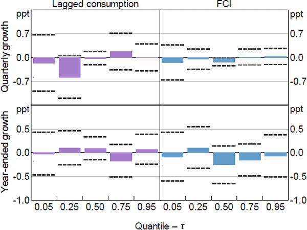
Note: Dashed lines represent 95 per cent confidence intervals computed using the stationary bootstrap proposed in Politis and Romano (1994) assuming an average block length of 8 quarters and 1,000 replications
Sources: ABS; Authors' calculations
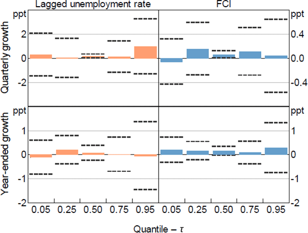
Note: Dashed lines represent 95 per cent confidence intervals computed using the stationary bootstrap proposed in Politis and Romano (1994) assuming an average block length of 8 quarters and 1,000 replications
Sources: ABS; Authors' calculations
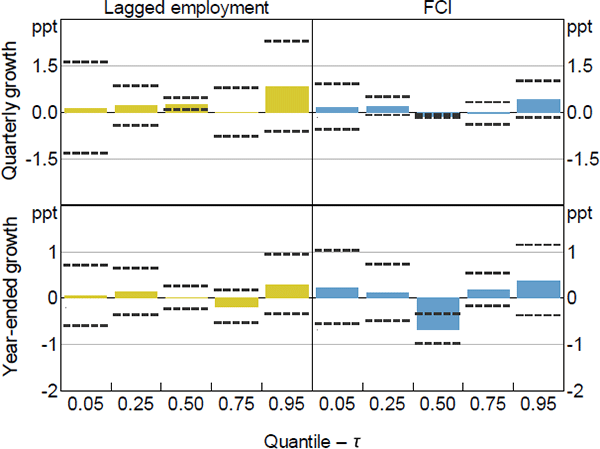
Note: Dashed lines represent 95 per cent confidence intervals computed using the stationary bootstrap proposed in Politis and Romano (1994) assuming an average block length of 8 quarters and 1,000 replications
Sources: ABS; Authors' calculations
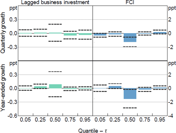
Note: Dashed lines represent 95 per cent confidence intervals computed using the stationary bootstrap proposed in Politis and Romano (1994) assuming an average block length of 8 quarters and 1,000 replications
Sources: ABS; Authors' calculations
B.2 Fitted quantile ranges
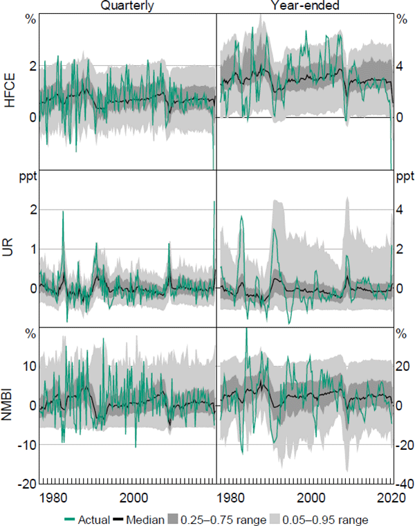
Notes: ‘HFCE’ is the growth rate of real household final consumption expenditure, actual HFCE quarterly growth rate for 2020:Q2 is –12.1 per cent, actual HFCE year-ended growth rate for 2020:Q2 is –12.8 per cent; ‘UR’ is the change in the total unemployment rate; ‘NMBI’ is the growth rate of real business investment excluding mining investment
Sources: ABS; Authors' calculations; RBA
B.3 Downside and upside risk estimates
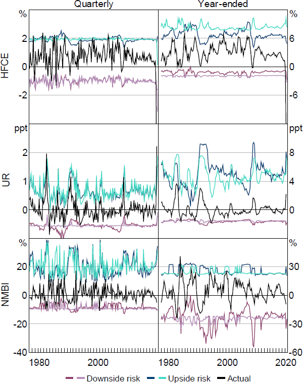
Notes: ‘HFCE’ is the growth rate of real household final consumption expenditure, actual HFCE quarterly growth rate for 2020:Q2 is –12.1 per cent, actual HFCE year-ended growth rate for 2020:Q2 is -12.8 per cent; ‘UR’ is the change in the total unemployment rate; ‘NMBI’ is the growth rate of real business investment excluding mining investment; is set equal to 5 per cent; thicker darker-coloured line is estimated with the FCI; thinner lighter-coloured line is estimated without the FCI
Sources: ABS; Authors' calculations; RBA
References
Adrian T, N Boyarchenko and D Giannone (2019), ‘Vulnerable Growth’, The American Economic Review, 109(4), pp 1263–1289.
Adrian T, F Grinberg, N Liang and S Malik (2018), ‘The Term Structure of Growth-at-Risk’, IMF Working Paper No WP/18/180.
Aikman D, J Bridges, S Burgess, R Galletly, I Levina, C O'Neill and A Varadi (2018), ‘Measuring Risks to UK Financial Stability’, Bank of England Staff Working Paper No 738.
Anderson BDO and JB Moore (1979), Optimal Filtering, Information and System Sciences Series, Prentice-Hall, New Jersey.
Azzalini A and A Capitanio (2003), ‘Distributions Generated by Perturbation of Symmetry with Emphasis on a Multivariate Skew t-distribution’, Journal of the Royal Statistical Society: Series B (Statistical Methodology), 65(2), pp 367–389.
Bańbura M and M Modugno (2014), ‘Maximum Likelihood Estimation of Factor Models on Datasets with Arbitrary Pattern of Missing Data’, Journal of Applied Econometrics, 29(1), pp 133–160.
Bank of Japan (2018), Financial System Report, October.
Bai J and K Li (2016), ‘Maximum Likelihood Estimation and Inference for Approximate Factor Models of High Dimension’, The Review of Economics and Statistics, 98(2), pp 298–309.
Bai J and S Ng (2002), ‘Determining the Number of Factors in Approximate Factor Models’, Econometrica, 70(1), pp 191–221.
Bai J and S Ng (2006), ‘Confidence Intervals for Diffusion Index Forecasts and Inference for Factor-Augmented Regressions’, Econometrica, 74(4), pp 1133–1150.
Bai J and S Ng (2013), ‘Principal Components Estimation and Identification of Static Factors’, Journal of Econometrics, 176(1), pp 18–29.
Bai J and P Wang (2015), ‘Identification and Bayesian Estimation of Dynamic Factor Models’, Journal of Business & Economic Statistics, 33(2), pp 221–240.
Barigozzi M and M Luciani (2019), ‘Quasi Maximum Likelihood Estimation and Inference of Large Approximate Dynamic Factor Models Via the EM Algorithm’, Unpublished manuscript, ver 1, October. Available at <https://arxiv.org/abs/1910.03821v1>.
Bordo MD and CM Meissner (2016), ‘Fiscal and Financial Crises’, in JB Taylor and H Uhlig (eds), Handbook of Macroeconomics: Volume 2A, Handbooks in Economics, Elsevier, Amsterdam, pp 355–412.
Brave S and RA Butters (2010), ‘Gathering Insights on the Forest from the Trees: A New Metric for Financial Conditions’, Federal Reserve Bank of Chicago Working Paper No 2010-07.
Buse A (1982), ‘The Likelihood Ratio, Wald, and Lagrange Multiplier Tests: An Expository Note’, The American Statistician, 36(3a), pp 153–157.
Carriero A, TE Clark and M Marcellino (2020), ‘Capturing Macroeconomic Tail Risks with Bayesian Vector Autoregressions’, Federal Reserve Bank of Cleveland Working Paper 20-02R, rev September.
Cecchetti SG (2006), ‘Measuring the Macroeconomic Risks Posed by Asset Price Booms’, NBER Working Paper No 12542.
Chodorow-Reich G (2014), ‘The Employment Effects of Credit Market Disruptions: Firm-Level Evidence from the 2008–09 Financial Crisis’, The Quarterly Journal of Economics, 129(1), pp 1–59.
Coroneo L, D Giannone and M Modugno (2016), ‘Unspanned Macroeconomic Factors in the Yield Curve’, Journal of Business & Economic Statistics, 34(3), pp 472–485.
Cryer JD and K-S Chan (2008), Time Series Analysis: With Applications in R, 2nd edn, Springer Texts in Statistics, Springer, New York.
Doz C, D Giannone and L Reichlin (2011), ‘A Two-Step Estimator for Large Approximate Dynamic Factor Models Based on Kalman Filtering’, Journal of Econometrics, 164(1), pp 188–205.
Doz C, D Giannone and L Reichlin (2012), ‘A Quasi–Maximum Likelihood Approach for Large, Approximate Dynamic Factor Models’, The Review of Economics and Statistics, 94(4), pp 1014–1024.
Duprey T and A Ueberfeldt (2018), ‘How to Manage Macroeconomic and Financial Stability Risks: A New Framework’, Bank of Canada Staff Analytical Note 2018-11.
Ellis L and C Naughtin (2010), ‘Commercial Property and Financial Stability – An International Perspective’, RBA Bulletin, June, pp 25–30.
European Central Bank (2018), Financial Stability Review, May.
Falconio A and S Manganelli (2020), ‘Financial Conditions, Business Cycle Fluctuations and Growth at Risk’, European Central Bank Working Paper Series No 2470.
Gauthier C, C Graham and Y Liu (2004), ‘Financial Conditions Indexes for Canada’, Bank of Canada Working Paper 2004-22.
Gebauer S, R Setzer and A Westphal (2018), ‘Corporate Debt and Investment: A Firm-Level Analysis for Stressed Euro Area Countries’, Journal of International Money and Finance, 86, pp 112–130.
Ghahramani Z and GE Hinton (1996), ‘Parameter Estimation for Linear Dynamical Systems’, Department of Computer Science, University of Toronto, Technical Report CRG-TR-96-2. Available at <https://www.cs.toronto.edu/~hinton/absps/tr96-2.html>.
Groen JJJ, MB Nattinger and AI Noble (2020), ‘Measuring Global Financial Market Stresses’, Federal Reserve Bank of New York Staff Report No 940.
Haldane AG (2009), ‘Rethinking the Financial Network’, Speech given at the Financial Student Association, Amsterdam, 28 April.
Hambur J and G La Cava (2018), ‘Do Interest Rates Affect Business Investment? Evidence from Australian Company-Level Data’, RBA Research Discussion Paper No 2018-05.
Hansen BE (1994), ‘Autoregressive Conditional Density Estimation’, International Economic Review, 35(3), pp 705–730.
Hatzius J, P Hooper, F Mishkin, KL Schoenholtz and MW Watson (2010), ‘Financial Conditions Indexes: A Fresh Look after the Financial Crisis’, in Financial Conditions Indexes: A Fresh Look after the Financial Crisis: Proceedings of the U.S. Monetary Policy Forum 2010, The Initiative on Global Markets, The University of Chicago Booth School of Business, Chicago, pp 3–59.
Kamber G, J Morley and B Wong (2018), ‘Intuitive and Reliable Estimates of the Output Gap from a Beveridge-Nelson Filter’, The Review of Economics and Statistics, 100(3), pp 550–566.
Kapetanios K, S Price and G Young (2017), ‘A UK Financial Conditions Index Using Targeted Data Reduction: Forecasting and Structural Identification’, Bank of England Staff Working Paper No 699.
Kearns J (2020), ‘Banking and the COVID-19 Pandemic’, Keynote address given at the 33rd Australasian Finance and Banking Conference, organised by the Institute of Global Finance and the School of Banking and Finance, UNSW Business School, Sydney, 15–17 December.
Kiley MT (2018), ‘Unemployment Risk’, Board of Governors of the Federal Reserve System Finance and Economics Discussion Series No 2018-067.
Koenker R (2005), Quantile Regression, Econometric Society Monographs, Cambridge University Press, Cambridge.
Loria F, C Matthes and D Zhang (2019), ‘Assessing Macroeconomic Tail Risk’, Board of Governors of the Federal Reserve System Finance and Economics Discussion Series No 2019-026.
Manzan S (2015), ‘Forecasting the Distribution of Economic Variables in a Data-Rich Environment’, Journal of Business & Economic Statistics, 33(1), pp 144–164.
Politis DN and JP Romano (1994), ‘The Stationary Bootstrap’, Journal of the American Statistical Association, 89(428), pp 1303–1313.
Prasad A, S Elekdag, P Jeasakul, R Lafarguette, A Alter, AX Feng and C Wang (2019), ‘Growth at Risk: Concept and Application in IMF Country Surveillance’, IMF Working Paper No WP/19/36.
Price F, B Beckers and G La Cava (2019), ‘The Effect of Mortgage Debt on Consumer Spending: Evidence from Household-Level Data’, RBA Research Discussion Paper No 2019-06.
Schmidt LDW and Y Zhu (2016), ‘Quantile Spacings: A Simple Method for the Joint Estimation of Multiple Quantiles without Crossing’, Working paper, 19 July. Available at <https://economics.sas.upenn.edu/events/quantile-spacings-simple-method-joint-estimation-multiple-quantiles-without-crossing>.
Simon J (2001), ‘The Decline in Australian Output Volatility’, RBA Research Discussion Paper No 2001-01.
Stock JH and MW Watson (2002), ‘Forecasting Using Principal Components from a Large Number of Predictors’, Journal of the American Statistical Association, 97(460), pp 1167–1179.
Stock JH and MW Watson (2016), ‘Dynamic Factor Models, Factor-Augmented Vector Autoregressions, and Structural Vector Autoregressions in Macroeconomics’, in JB Taylor and H Uhilg (eds), Handbook of Macroeconomics: Volume 2A, Handbooks in Economics, Elsevier, Amsterdam, pp 415–525.
Wu LS-Y, JS Pai and JRM Hosking (1996), ‘An Algorithm for Estimating Parameters of State-Space Models’, Statistics & Probability Letters, 28(2), pp 99–106.
Zdzienicka A, S Chen, F Diaz Kalan, S Laseen and K Svirydzenka (2015), ‘Effects of Monetary and Macroprudential Policies on Financial Conditions: Evidence from the United States’, IMF Working Paper No WP/15/288.
Copyright and Disclaimer Notice
RP Data Pty Ltd trading as CoreLogic Asia Pacific Disclaimer Notice
The following Disclaimer Notice applies to content that uses data from CoreLogic:
This publication contains data, analytics, statistics, results and other information licensed to the Reserve Bank of Australia by RP Data Pty Ltd trading as CoreLogic Asia Pacific (CoreLogic Data).
© Copyright 2021. RP Data Pty Ltd trading as CoreLogic Asia Pacific (CoreLogic) and its licensors are the sole and exclusive owners of all rights title and interest (including intellectual property rights) subsisting in the CoreLogic Data reproduced in this publication. All rights reserved.
The CoreLogic Data provided in this publication is of a general nature and should not be construed as specific advice or relied upon in lieu of appropriate professional advice.
While CoreLogic uses commercially reasonable efforts to ensure the CoreLogic data is current, CoreLogic does not warrant the accuracy, currency or completeness of the CoreLogic Data and to the full extent permitted by law excludes all loss or damage howsoever arising (including through negligence) in connection with the CoreLogic Data.
Acknowledgements
We are grateful to Benjamin Beckers, Michele Bullock, Jonathan Kearns, Jeffrey Sheen, John Simon, Penelope Smith, seminar participants at the Reserve Bank of Australia, workshop participants at the Sydney Macroeconomic Reading Group Workshop, seminar participants at the University of Queensland, conference participants at the 3rd Sydney Banking and Financial Stability Conference held at the University of Sydney in December 2019 as well as workshop participants at the DBS-SWUFE Centre for Banking and Financial Stability Workshop held at Deakin University in February 2020 for helpful comments and suggestions. We would also like to thank Lawrence Schmidt for useful discussions related to understanding and implementing the quantile spacing method as well as Mark Phoon and Marcus Miller for data assistance. Any remaining errors are solely our own. The views expressed in this paper are those of the authors and do not necessarily reflect the views of the Reserve Bank of Australia.
Footnotes
In a recent paper, Falconio and Manganelli (2020) suggest that controlling for economic risk eliminates the direct effect of financial shocks on the real economy. This suggests that financial shocks instead have an indirect effect on the real economy via their effect on economic uncertainty. [1]
We use a continuous distribution because computing the area in the tails requires us to use (numerical) integration. [2]
An additional technical reason for preferring expected shortfall over VaR is that it is a ‘coherent’ measure of risk while VaR is not. This is because VaR violates the sub-additivity property. [3]
We convert any series available at higher frequencies to a quarterly frequency by computing the quarter average for ‘flow’ variables or using the quarter-ended value for ‘stock’ variables. [4]
The FCI developed by Hatzius et al (2010) for the United States is also quarterly. [5]
The estimated FCI for September quarter 2020 includes only 42 of the 75 variables owing to data availability at the time of estimation. [6]
There is no clear convention regarding the sign of the FCI, but we follow the Federal Reserve Bank of Chicago in defining more restrictive conditions with positive values and expansionary conditions with negative values. Appendix A.2 describes how we implement this specific sign convention when estimating the FCI. [7]
The narrowness of the estimated confidence interval is related to the number of variables in our dataset ( N ), which is large relative to the number of observations for each variable ( T ). [8]
In an empirical application related to forecasting the distribution of stock returns, Schmidt and Zhu (2016) show that their method outperforms the standard QR method for most quantiles, especially on the lower tail of the distribution. They suggest this could translate into a better estimate for tail measures such as VaR. [9]
A second issue with standard QR discussed in Carriero et al (2020) concerns estimating tail quantiles with small sample sizes. The problem relates to quantile estimates that can be seen as unrealistically extreme. The quantile spacing method is also susceptible to this issue given the use of the exponential function in Equation (2). To mitigate this problem we use a form of winsoring when constructing the quantile estimates. [10]
In the quantile spacing setting, Schmidt and Zhu (2016) suggest these particular values will also characterise the effect of a one unit change in our explanatory variables on the width of the left tail, left shoulder (i.e. the area between the peak of the distribution and the tail), right shoulder and right tail of the distribution. [11]
This distribution is very flexible and nests other well-known distributions, including the Gaussian, Laplace, Student's t or Cauchy. [12]
This ST specification differs to Adrian et al (2019) who use the ST distribution developed by Azzalini and Capitanio (2003). We chose the version proposed by Hansen (1994) for computational reasons. [13]
The parameters of the ST distribution have the following restrictions: and q > 0. If the ST becomes the Student's t distribution. If the ST becomes a skewed Gaussian distribution. If and the ST becomes the Gaussian distribution. [14]
We employ parameter transformations on and when solving the minimisation problem to the ensure the ST parameter restrictions are enforced. [15]
The 95 per cent confidence intervals were constructed from bootstrapped standard errors using the stationary bootstrap developed in Politis and Romano (1994), assuming an average block length of 8 quarters and 1,000 replications. Note, we computed the standard errors in this way because the bootstrap methods proposed in Schmidt and Zhu (2016) ignore any potential serial correlation that might be present in the data. [16]
More specifically, it is the average of all estimated outcomes below the 0.05 quantile of the fitted distribution. [17]
This decision also has a practical purpose. We initialise our DFM using parameter estimates derived from principal components analysis which requires a balanced dataset. Hence, a dataset with lots of very short series could result in less precise starting values which will affect the estimation of the FCI. [18]
Variables are made stationary by taking logs and/or differences as appropriate. [19]
This will also be useful to correct for any structural drift in the mean of any series as well. [20]
Bai and Wang regard the specification to be a static factor model when there are no lags in the measurement equation (i.e. s = 0). [21]
Note, this information criterion is only designed to be used to determine the number of static factors in a dataset and not the number of dynamic factors in a dataset. Our dynamic factor model with one factor and one lag can be rewritten as a static factor model with 2 factors. As a robustness check we test whether the inclusion of the lag (i.e. the second static factor) is supported by the data and we find that it is. These results are in Appendix A.4. [22]
Estimation is ‘quasi’ maximum likelihood because the model is misspecified. This comes from assuming that R the covariance matrix of the idiosyncratic component is diagonal. Additionally, we also assume that both noise processes are Gaussian. However, in large samples, this has been shown to be no issue (see Doz et al (2012), Bai and Li (2016) and Barigozzi and Luciani (2019)). [23]
The identifying restriction ‘DFM2’ is similar to the identifying restrictions ‘PC3’ suggested by Bai and Ng (2013) and ‘IC1’ suggested by Bai and Li (2016). [24]
Our decision to use the LR test relies on Bai and Wang (2015)'s suggestion that a Wald test for parameter restrictions in the DFM is feasible and a Wald test is asymptotically equivalent to a LR test (see Buse (1982)). [25]
The original frequency of the unemployment rate and the employment series is monthly. We convert both series to a quarterly frequency by taking the quarter-ended monthly value. [26]
We chose to use a maximum of 4 lags based on sample cross-correlation analysis in Table A2. [27]