RDP 2023-01: The Effect of Credit Constraints on Housing Prices: (Further) Evidence from a Survey Experiment 8. Interpreting the Experimental Results with a User Cost Model
January 2023
- Download the Paper 1.55MB
The non-parametric demand curve analysis used above estimates the effect of financing conditions on the marginal buyer's WTP, and shows the difference between it and the average WTP change. But it cannot say much about the why the marginal buyer and the average diverge. My explanation is that more responsive households are responsive because they are more constrained and have WTPs below the market price, which means they are less likely to bear on the market price. The user cost model of housing demand, presented in Fuster and Zafar (2021) and adapted here for heterogeneity, can give a more precise description of the mechanisms involved.
8.1 Standard user cost model
Fuster and Zafar (2021) consider the response of WTPs to the easing of collateral constraints through the lens of a standard user cost model as set out in Glaeser, Gottlieb and Gyourko (2012) and reprinted below as Equation (1). The idea of the user cost model is that a household compares the present value of the costs of renting a home and buying the same home, then chooses whichever is cheaper. For the marginal buyer, the costs of renting and buying should be equal in equilibrium, which means the user cost as a fraction of price should equal the rent-to-price ratio.
: down payment fraction
: subjective discount rate
: mortgage rate after tax deduction, where is marginal tax rate
: property taxes, maintenance, insurance (as a fraction of price)
g : growth rate of rent
: mobility rate.
Assuming fixed rent and supply, Fuster and Zafar (2021, p 237) note that ‘the elasticity of the equilibrium price thus corresponds to the elasticity of demand, which is what we will measure in our survey’. They measure average elasticity, but the elasticity of the marginal buyer determines price changes. These will coincide if all market participants have the same elasticity, but the heterogeneity in responses shows that is not the case. Fuster and Zafar do report different average elasticities within subgroups – most notably renters versus owners – but as demonstrated by the analysis of market segments in Section 6 households within segments show important heterogeneity and the elasticity of many individuals' demand is irrelevant to market pricing.
8.2 A heterogeneous user cost model
Recognising that not all WTPs influence market pricing calls for a slightly altered heterogeneous user cost model. I adapt the standard user cost framework to include an idiosyncratic discount rate for each household, i (Equation (2)). Relaxing the representative agent assumption breaks the direct mapping from demand to price, so the equation is now specified as a WTP for each household rather than the price. Further mapping to the price requires considering who is marginal.
The subjective discount rate is an important dimension of heterogeneity but is unlikely to be the only one, and it cannot account for all the variation in the data. In principle, any element of the user cost model can be heterogeneous. Previous modelling research on the rent versus buy decision often includes a rental preference parameter, for example, Corbae and Quintin (2015), Kaplan et al (2020) and Greenwald and Guren (2021). To keep the model simple and engage with that literature, I add a rent versus own preference parameter, , to the user cost model. For > 0 the household is willing to pay more than the discounted sum of rent to own the house, and vice versa for < 0. For all other parameters in the user cost equation I use the calibration from Fuster and Zafar (2021).
Conditional on the calibrated cost parameters, Equation (2) shows how the preference parameters determine both the ratio of a household's WTP to the rent on a home, as well as the elasticity of the WTP to a change in collateral constraints. The level of the WTP is determined by both the rent versus own parameter, , and the subjective discount rate parameter, . The response to collateral constraint changes is determined only by because WTP is linear in . Figure 8 shows the WTP-to-rent ratio as a function of , assuming = 0 (i.e. indifference between owning and renting), a before-tax mortgage rate of 5.5 per cent, and using the Fuster and Zafar (2021) calibration for the cost parameters.[7] The WTP is steeply decreasing in as the household increasingly discounts the value of future imputed rents.
The lower panel of Figure 8 shows the response of a household's theoretical WTP to the experimental changes of loosening the collateral constraint and cutting the interest rate. The response of WTP to collateral increases sharply in . If a household's subjective discount rate is equal to the after-tax mortgage rate (3.6 per cent in this example), then the WTP response is zero, climbing to a log change of 0.3 at a discount rate of 20 per cent. The response of WTP to a change in interest rate is little changed across the spectrum of subjective discount rates.
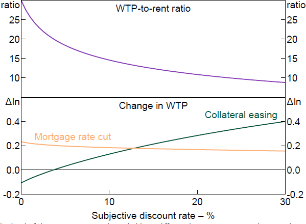
Note: The level of the WTP assumes a household is indifferent between owning and renting (i.e. = 0), while the change is independent of .
The heterogeneous discount rate is written in Equation (2) as a preference parameter, but it can be thought of as combining genuine preference heterogeneity with differences in circumstances. The key circumstance is likely to be the household's available financial resources compared to the collateral required for their home. That said, household preferences are likely to affect accumulation of financial resources, which makes it difficult to disentangle preferences and circumstances without a more detailed model. To avoid taking a stand on the behavioural mechanism and let the experimental data speak for itself, I combine circumstances and preferences into one parameter. Similarly, the rent versus buy parameter is likely to be influenced by life-cycle factors as well as deeper preferences.
8.3 Mapping the data to the heterogeneous user cost model
The heterogeneous user cost equation in Equation (2) creates a mapping from the WTP data onto the discount rate and rent versus buy preference parameters. A similar approach was taken in Alvarez and Argente (2020) to model heterogeneity in a very different experimental setting about using cash for payments. For the Fuster and Zafar (2021) experiment, each WTP question for each household gives an instance of Equation (2) with different values for WTPi , and r. From there, the equations can be solved for the preference parameters, and , for each household.[8]
Equation (2) also includes the rent of each dwelling, which is not observed. The discount rate, , can be identified from the ratio of WTPs in the two down payment scenarios, which means it does not depend on rent. Because a household's WTP is linear in the rent versus own preference parameter, , it cancels out within the ratio. Identifying does require the rent of each dwelling. To proxy for rent, I multiply the home value by the rent-to-price ratio implied by the Fuster and Zafar (2021) calibration of the user cost model with the discount rate equal to the mortgage rate.
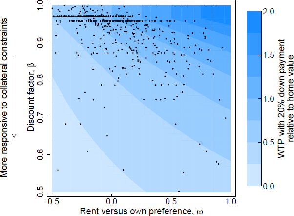
Figure 9 shows a scatter plot of the joint distribution of the preference parameters inferred from the WTP data overlaid on the theoretical relationship of the two parameters with the level of WTP.[9] With two dimensions of heterogeneity it is possible for households with a high initial WTP to be very responsive to changes in down payment restrictions. Such a household would have a high discount rate, , possibly due to financial constraints, and a strong preference to own rather than rent. This region of the preference space corresponds to the lower right region of Figure 9. A market segment including many households within this region would exhibit both a responsive marginal WTP and a responsive average WTP. In the data this area is sparsely populated, which is consistent with the direct analysis of demand curves – the large increases in WTP are mostly at the lower end of the normalised WTP spectrum in levels.
Notes
The contours in the figure show the theoretical relationship between WTP and the preference parameters with 20 per cent down payment. Each dot shows the preference parameter inferred from a household's WTPs.
(a) I transform the interest-rate-equivalent subjective discount rate to a subjective discount factor They can be used equivalently in the user cost model but is easier to visualise because WTPs close to zero map to values close to zero and values approaching infinity.
Sources: Author's calculations; Fuster and Zafar (2021)
Footnotes
In the United States, mortgage interest is tax deductible up to a limit. [7]
I solve for the preference parameters using WTPs from first two questions (i.e. just using the two down payment conditions). Results are similar if I include the third question with a different interest rate and fit the two preference parameters by maximum likelihood. I do not consider the inheritance condition because it does not map as well to the user cost model. [8]
Appendix C.1 shows the distribution of each parameter individually. [9]