Bivariate Example | RDP 2023-07: Identification and Inference under Narrative Restrictions

RDP 2023-07: Identification and Inference under Narrative Restrictions 2. Bivariate Example

Raffaella Giacomini, Toru Kitagawa and Matthew Read

October 2023

Download the Paper 1.10MB

We illustrate the econometric issues that arise when imposing NR in the context of the following bivariate SVAR(0): $A_{0} y_{t} = ε_{t}$ , for t = 1,…,T, where y_t = (y_1t, y_2t)′ and $ε_{t} = {(ε_{1 t}, ε_{2 t})}^{'}$ , with $ε_{t}^{_{\sim}^{i i d}} N (0_{2 \times 1}, I_{2})$ . We abstract from dynamics for ease of exposition, but this is without loss of generality. The orthogonal reduced form of the model reparameterises A₀ as $Q^{'} \sum_{t r}^{- 1}$ , where $\sum_{t r}$ is the lower-triangular Cholesky factor (with positive diagonal elements) of $\sum = 𝔼 (y_{t} {y^{'}}_{t}) = A_{0}^{- 1} {(A_{0}^{- 1})}^{'}$ . We parameterise $Σ_{t r}$ as

(1)

Σ_{t r} = [\begin{matrix} σ_{11} & 0 \\ σ_{12} & σ_{22} \end{matrix}] (σ_{11}, σ_{22} > 0)

and denote the vector of reduced-form parameters as $ϕ = vech (Σ_{t r})$ . Q is an orthonormal matrix in the space of 2×2 orthonormal matrices, $𝒪$ (2):

(2)

Q \in 𝒪 (2) = {[\begin{matrix} \cos θ & - \sin θ \\ \sin θ & \cos θ \end{matrix}]} \cup {[\begin{matrix} \cos θ & \sin θ \\ \sin θ & - \cos θ \end{matrix}]}

where $θ \in [- π, π]$ . This formulation of the model, which follows Baumeister and Hamilton (2015), means that the structural parameters can be expressed as functions of the reduced-form parameters and $θ$ . Restrictions on the structural parameters and/or functions of the structural shocks can then be interpreted as restricting $θ$ to some set. In what follows, we discuss properties of this set that are key for analysing identification and inference under NR.

2.1 Shock-sign restrictions

Consider the ‘shock-sign restriction’ that $ε_{1 k}$ is non-negative for some $k \in {1, ..., T}$ :

(3)

ε_{1 k} = {e^{'}}_{1, 2} A_{0} y_{k} = {(σ_{11} σ_{22})}^{- 1} (σ_{22} y_{1 k} \cos θ + (σ_{11} y_{2 k} - σ_{21} y_{1 k}) \sin θ) \geq 0

Equation (3) implies that the restricted structural shock can be written as a function $ε_{1 k} (θ, ϕ, y_{k})$ . Along with the ‘sign normalisation’ $diag (A_{0}) \geq 0_{2 \times 1}$ , the shock-sign restriction implies that $θ$ is restricted to the set

(4)

\begin{array}{l} θ \in {θ : σ_{21} \sin θ \leq σ_{22} \cos θ, \cos θ \geq 0, σ_{22} y_{1 k} \cos θ \geq (σ_{21} y_{1 k} - σ_{11} y_{2 k}) \sin θ} \\ \cup {θ : σ_{21} \sin θ \leq σ_{22} \cos θ, \cos θ \leq 0, σ_{22} y_{1 k} \cos θ \geq (σ_{21} y_{1 k} - σ_{11} y_{2 k}) \sin θ} \end{array}

The restriction induces a set-valued mapping from $ϕ$ to $θ$ that depends on the realisation of y_k. Giacomini et al (2022a) characterise this mapping in the case where $σ_{21} < 0$ . For example, if $h (ϕ, y_{k}) = σ_{21} y_{1 k} - σ_{11} y_{2 k} < 0$ , then

(5)

θ \in [\arctan (\max {\frac{σ_{22}}{σ_{21}}, C (ϕ, y_{k})}), π + \arctan (\min {\frac{σ_{22}}{σ_{21}}, C (ϕ, y_{k})})]

where $C (ϕ, y_{k}) = σ_{22} y_{1 k} / h (ϕ, y_{k})$ . The direct dependence of this mapping on the realisation of the data implies that the standard notion of an identified set – the set of observationally equivalent structural parameters given the reduced-form parameters – does not apply. Consequently, it is not obvious whether the restrictions are, in fact, set identifying in a formal frequentist sense, nor whether existing frequentist procedures for conducting inference in set-identified models are valid. We analyse identification under these restrictions in Section 4.

When conducting Bayesian inference, AR18 construct the posterior using the conditional likelihood – the likelihood of observing the data conditional on the NR holding. Letting $y^{T} = {({y^{'}}_{1}, ..., {y^{'}}_{T})}^{'}$ , the conditional likelihood is

(6)

p (y^{T} | θ, ϕ, ε_{1 k} (θ, ϕ, y_{k}) \geq 0) = \frac{Π_{t = 1}^{T} {(2 π)}^{- 1} {| Σ |}^{- \frac{1}{2}} \exp (- \frac{1}{2} {y^{'}}_{t} Σ^{- 1} y_{t})}{\Pr (ε_{1 k} \geq 0 | θ, ϕ)} 1 (ε_{1 k} (θ, ϕ, y_{k}) \geq 0)

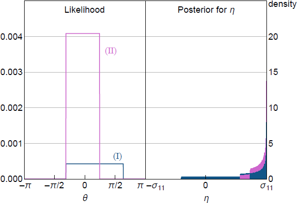
The denominator in the first term – the ex ante probability that the NR is satisfied – equals ½, because $ε_{1 k}$ is standard normal. The conditional likelihood therefore depends on $θ$ only through the indicator function $1 (ε_{1 k} (θ, ϕ, y_{k}) \geq 0)$ , which truncates the likelihood, with the truncation points depending on y_k. To illustrate, the left panel of Figure 1 plots the conditional likelihood as a function of $θ$ given two realisations of a data-generating process and fixing $ϕ$ to its true value.^[5] The conditional likelihood is flat over the interval for $θ$ satisfying the shock-sign restriction and is zero outside this interval. The support of the non-zero region depends on y_k.

Figure 1: Shock-sign Restriction in Bivariate Model

The flat likelihood implies that the posterior for $θ$ is proportional to the prior in the region where the likelihood is non-zero, and is zero outside this region. The standard approach to Bayesian inference in SVARs under sign restrictions assumes a uniform prior over Q, as do AR18.^[6] In the bivariate example, this is equivalent to a prior for $θ$ that is uniform (Baumeister and Hamilton 2015). This prior implies that the posterior for $θ$ is also uniform over the interval for $θ$ where the likelihood is non-zero.

The impact impulse response of y_1t to a positive standard deviation shock $ε_{1 t}$ is $η \equiv σ_{11} \cos θ$ . The right panel of Figure 1 plots the posterior for $η$ induced by a uniform prior over $θ$ given the same realisations of the data for which the likelihood was plotted in the left panel. It can be seen that the posterior for $η$ assigns more probability mass to more-extreme values of $η$ . This highlights that even a uniform prior may be informative for parameters of interest, which also occurs under traditional sign restrictions (Baumeister and Hamilton 2015). One difference is that the prior under sign restrictions is never updated by the data, whereas the support and shape of the posterior for $η$ under NR may depend on the realisation of y_k through its effect on the truncation points of the likelihood, so there may be some updating of the prior. However, the prior is not updated at values of $θ$ corresponding to the flat region of the likelihood. Posterior inference about $η$ may therefore still be sensitive to the choice of prior, as in standard set-identified SVARs.

2.2 Historical decomposition restrictions

The historical decomposition is the contribution of a particular structural shock to the observed unexpected change in a particular variable over some horizon. The contribution of the first shock to the change in the first variable in the kth period is

(7)

H_{1, 1, k} (θ, ϕ, y_{k}) = σ_{22}^{- 1} (σ_{22} y_{1 k} \cos^{2} θ + (σ_{11} y_{2 k} - σ_{21} y_{1 k}) \cos θ \sin θ)

while the contribution of the second shock is

(8)

H_{1, 2, k} (θ, ϕ, y_{k}) = σ_{22}^{- 1} (σ_{22} y_{1 k} \sin^{2} θ + (σ_{21} y_{1 k} - σ_{11} y_{2 k}) \cos θ \sin θ)

Consider the restriction that the first structural shock in period k was positive and (in the language of AR18) the ‘most important contributor’ to the change in the first variable, which requires that $| H_{1, 1, k} (θ, ϕ, y_{k}) | \geq | H_{1, 2, k} (θ, ϕ, y_{k}) |$ . Under these restrictions, $θ$ must satisfy a set of inequalities that depends on $ϕ$ and y_k. As in the case of the shock-sign restriction, this set of inequalities generates a set-valued mapping from $ϕ$ to $θ$ that depends on y_k.

Let $D (θ, ϕ, y_{k}) = 1 {ε_{1 k} (θ, ϕ, y_{k}) \geq 0, | H_{1, 1, k} (θ, ϕ, y_{k}) | \geq | H_{1, 2, k} (θ, ϕ, y_{k}) |}$ represent the indicator function equal to one when the NR are satisfied and equal to zero otherwise, and let $\tilde{D} (θ, ϕ, ε_{k}) = 1 {ε_{1 k} \geq 0, | {\tilde{H}}_{1, 1, k} (θ, ϕ, ε_{1 k}) | \geq | {\tilde{H}}_{1, 2, k} (θ, ϕ, ε_{2 k}) |}$ denote the indicator function for the same event in terms of the structural shocks rather than the data. The conditional likelihood given the restrictions is then

(9)

p (y^{T} | θ, ϕ, D (θ, ϕ, y_{k}) = 1) = \frac{Π_{t = 1}^{T} {(2 π)}^{- \frac{n}{2}} {| Σ |}^{- \frac{1}{2}} \exp (- \frac{1}{2} {y^{'}}_{t} Σ^{- 1} y_{t})}{\Pr (\tilde{D} (θ, ϕ, ε_{k}) = 1 | θ, ϕ)} D (θ, ϕ, y_{k})

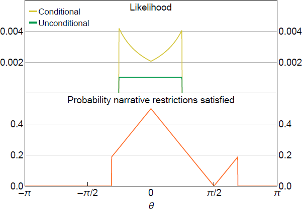
In contrast to the case of shock-sign restrictions, the probability in the denominator now depends on $θ$ through the historical decomposition. Intuitively, changing $θ$ changes the impulse responses of y_1t to the two shocks and thus changes the ex ante probability that $| {\tilde{H}}_{1, 1, k} (θ, ϕ, ε_{1 k}) | \geq | {\tilde{H}}_{1, 2, k} (θ, ϕ, ε_{2 k}) |$ . Consequently, the likelihood is not necessarily flat when it is non-zero.

To illustrate, the top panel of Figure 2 plots the conditional likelihood under the historical decomposition NR using the same data-generating process as in Figure 1. The bottom panel plots the probability in the denominator of the conditional likelihood. The likelihood is again truncated, but it is no longer flat – it has a maximum at the value of $θ$ that minimises the ex ante probability that the NR are satisfied (within the set of values of $θ$ that are consistent with the restriction given the realisation of the data). The posterior for $θ$ induced by the usual uniform prior will therefore assign greater posterior probability to values of $θ$ that yield a lower ex ante probability of satisfying the NR.

Figure 2: Historical Decomposition Restriction in Bivariate Model

If we view the narrative event ( $i .e . \tilde{D} (θ, ϕ, ε_{k})$ ) as observable and its probability of occurring depends on the parameter of interest, then conditioning on the narrative event implies that we are conditioning on a non-ancillary statistic. This is undesirable when conducting likelihood-based inference, because it represents a loss of information about the parameter of interest. Unlike for the shock-sign restriction, the probability that the historical decomposition restriction is satisfied depends on $θ$ , so the event that the NR are satisfied is not ancillary. Conditioning on this event means that the shape of the likelihood (within the non-zero region) is fully driven by the inverse probability of the conditioning event.

Based on this consideration, we therefore advocate constructing the posterior using the joint (or unconditional) likelihood of observing the data and the NR holding:

(10)

p (y^{T}, D (θ, ϕ, y_{k}) = 1 | θ, ϕ) = \prod_{t = 1}^{T} {(2 π)}^{- 1} {| Σ |}^{- \frac{1}{2}} \exp (- \frac{1}{2} {y^{'}}_{t} Σ^{- 1} y_{t}) D (θ, ϕ, y_{k})

For all types of NR, the unconditional likelihood is flat with respect to $θ$ (when it is non-zero) and depends on $θ$ only through the points of truncation. Of course, this means that posterior inference based on the unconditional likelihood may be sensitive to the choice of prior, as when using the conditional likelihood under shock-sign restrictions. In Section 5.2, we propose how to deal with this posterior sensitivity.

Footnotes

The data-generating process assumes vec(A₀) = (1,0.2,0.5,1.2)′, which implies that $σ_{21} < 0$ and $θ = \arcsin (0.5 σ_{22})$ with Q equal to the rotation matrix. We assume the time series is of length T = 3 and draw sequences of structural shocks such that $ε_{1, 1} \geq 0.$ T is a small number to control Monte Carlo sampling error. The analysis with $ϕ$ set to its true value replicates the situation with a large sample, where the likelihood for $ϕ$ concentrates at the truth. It also facilitates visualising the likelihood, which otherwise is a function of four parameters. [5]

See, for example, Uhlig (2005), Rubio-Ramírez, Waggoner and Zha (2010) and Arias, Rubio-Ramírez and Waggoner (2018). [6]