Research Discussion Paper – RDP 2024-08 Modelling Reserve Demand with Deposits and the Cost of Collateral
1. Introduction
Central bankers in Australia and overseas are actively considering how best to design their monetary policy implementation system – the method by which they control short-term interest rates. Deposits held by commercial banks at the central bank – known as reserves – play an essential role in how the Reserve Bank of Australia (RBA) achieves interest rate control. Commercial banks are required to use reserves to settle payments with one another and the RBA. When a bank has insufficient reserves to settle their payments, they can borrow for a short time from other banks. The volume-weighted interest rate on these transactions is the cash rate – the RBA's interest rate target.
In Australia, the supply of reserves has declined as unconventional policies enacted during COVID-19 unwind, prompting discussion over the appropriate steady-state supply of reserves. To this end, the RBA recently announced it will operate an ‘ample reserves’ system where it supplies as many reserves as banks demand through open market operations (OMO) repo. The European Central Bank, Bank of England and Sweden's Riksbank have announced they will operate similar systems (Schnabel 2024; Ramsden 2018; Sveriges Riksbank 2019). This system is often referred to as a ‘demand-driven’ system because the value of reserves supplied by the central bank is determined by the banking system's demand, subject to the price set by the central bank.
I estimate Australian banks' reserve demand curve and its drivers. This is important for two reasons. First, banks' reserve demand will be an important determinant of the size of the RBA's balance sheet and its presence in financial markets. Second, the supply of reserves has been above the level banks would willingly hold at the price offered by the RBA since unconventional monetary policy measures were enacted during the COVID-19 pandemic. As unconventional policy unwinds, the supply of reserves will eventually fall to a point close to banks' underlying demand. At this point, banks will begin to demand additional reserves through the RBA's OMO, marking the transition from abundant reserves to its chosen system of ample reserves. Understanding banks' reserve demand aids in anticipating the timing of the transition.
There are two novel features of my work. First, I study reserve demand in the Australian context for the first time. Second, I model the time-varying cost of collateral and estimate its effect on the demand for reserves.
My work is closest to Lopez-Salido and Vissing-Jørgensen (2024), as I use their convenience yield framework to model the demand for reserves. Their focus is, however, on the US context, and in modelling reserve demand with respect to the overnight unsecured rate. I focus on the Australian context and overnight repo rate due to institutional features in Australian short-term money markets.
Given the RBA's current OMO price, my results suggest banks will demand somewhere between $100 billion and $200 billion of excess reserves (reserves held over and above minimum requirements imposed by the RBA).[1] Taking these estimates at face value, the RBA will be required to inject significantly more reserves to implement monetary policy than prior to the COVID-19 pandemic, when excess reserves averaged around $3 billion. Partly, what appears likely to be an increase in Australian banks' reserve demand reflects a decrease in the cost of borrowing under repo from OMO – a movement along banks' reserve demand curve. I find an increase in banking system deposits can explain a large part of the increase in reserve demand – a shift to the right in Australian banks' reserve demand curve. A shift in banks' reserve demand is not unique to Australia: existing research has documented the phenomenon in many jurisdictions including the euro area, the United Kingdom and the United States (Vissing-Jørgensen 2023; Meinecke 2023; Lopez-Salido and Vissing-Jørgensen 2024). The explanatory power of deposits suggests banks are willing to pay for the convenience of holding additional reserves to manage payments between depositors or that banks hold a precautionary reserve buffer against deposits in case of a liquidity stress.
Illustrating the high degree of uncertainty in estimating reserve demand, the supply of reserves at 30 October 2024 is around the upper range of my estimates while projections for the supply of reserves do not reach the lower range of my estimates until late 2026.[2]
The paper proceeds as follows. Section 2 provides background to establish how reserve demand might have changed since the COVID-19 pandemic. Section 3 outlines literature which addresses the challenges in estimating reserve demand. Section 4 presents a conceptual framework for the motivations behind banks' reserve demand which informs the data and modelling choices in Sections 5 and 6. Section 7 presents results from the modelling exercise, the implications of which are discussed in Section 8.
2. Background
Prior to the COVID-19 pandemic, the RBA supplied just enough reserves (around $3 billion) for banks to settle their interbank payments by the end of the day, known as a ‘scarce reserves’ system. Under scarce reserves, the RBA managed the supply of reserves to closely match demand such that the cash rate traded at target. While the cash rate traded at target, the overnight general collateral (GC) repo rate traded 10 to 20 basis points above cash rate. The difference in overnight rates represented a lack of arbitrage due to balance sheet limitations and because banks were less willing to lend in the repo market in the morning, wary that they may not be able to borrow back these funds in the cash market at the end of the trading day (Cheung and Printant 2019; Bristow and Tang 2024). The cash rate was also prevented from rising alongside repo rates due to a convention by cash market participants to almost always trade at the cash rate target (Kent 2024).
During the pandemic, the RBA ceased actively managing the supply of reserves when it began fulfilling all bids for liquidity at its OMO, purchased a large number of bonds and initiated the Term Funding Facility (TFF) (Debelle 2021). In doing so, the supply of reserves increased such that the cash and overnight GC repo rates converged on the interest paid on reserves – known as the ‘ES (exchange settlement) rate’ (Figure 1).
Since 2023, reserves have declined to around $200 billion from their peak of $450 billion as the RBA's bond purchases have begun to unwind and the TFF was repaid in full. While reserves remain at a high level relative to pre-pandemic, the decline in reserves has coincided with an increase in the cash and overnight repo rates (relative to the ES rate). The decline in reserves has revealed a time-varying relationship between the level of reserves and the spread between the overnight repo rate and the ES rate, akin to a shift in banks' reserve demand (Figure 2).
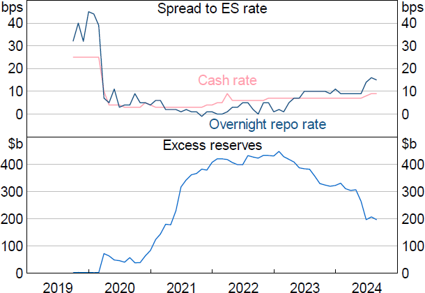
Sources: APRA; Author's calculations; RBA.
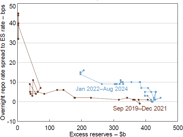
Sources: APRA; Author's calculations; RBA.
3. Literature Review
The literature identifies three unique features about the demand curve for reserves and several techniques for estimation consistent with these features.
First, it is highly nonlinear. The reserve demand curve is frequently drawn as kinked or roughly hyperbolic around a certain high level of reserves – known as the ‘saturation’ point (Frost 1971; Reis 2016). Beyond the saturation point banks are no longer willing to pay above the ES rate to obtain more reserves. The literature assumes various functional forms which differ in the degree to which market rates rise as reserves decline from their saturation point, including: log, hyperbolic, logistic, double exponential and arctangent (Nicolae 2020; Veyrune, della Valle and Guo 2018; Smith 2021; Bräuning 2018; Chen, Kourentzes and Veyrune 2023). In support of the log functional form, Lopez-Salido and Vissing-Jørgensen (2024) derive a microfoundation of the convenience yield of reserves in which reserves enter in logs. The logistic functional form is unique among the related literature as it assumes an upper asymptote as reserves decline toward zero. Veyrune et al (2018) impose the upper asymptote at the lending facility rate due to a lack of observed data close to this rate – a strong identifying assumption which presupposes an absence of stigma at the lending facility.
Second, banks' demand curve for reserves has been shown to shift over time. To document a shift, one strand of the literature estimates the demand curve separately for distinct time periods such as during central bank balance sheet expansion and unwind (Aberg et al 2021; Smith 2021). Another strand uses high-frequency data and rolling time periods to estimate the slope of the demand curve over time (Afonso et al 2022; Smith and Valcaral 2023). Both approaches are useful in documenting shifts in the demand curve and in monitoring how steep the slope of the demand curve is in real time (Afonso et al 2024). They do not, however, explain why the demand curve has shifted. Using US data, Lopez-Salido and Vissing-Jørgenson (2024) confirm empirically that liquid deposits shift banks' demand curve in an ample reserves system. They conclude that banks are willing to pay for additional reserves if they reduce transaction costs associated with managing a higher volume of payments between depositors, or in other words additional reserves generate a ‘convenience yield’. The finding that liquid deposits shift banks' demand curve holds when replicated using UK and euro area data but not Canadian (Meinecke 2023; Vissing-Jørgensen 2023; Bulusu et al 2023). Using US data, Acharya et al (2023) find that credit lines are statistically significant, in addition to liquid deposits, when explaining a shift in reserve demand. The mechanism for credit lines affecting demand is conceptually similar to liquid deposits but credit lines emphasise the importance of banks' holding precautionary buffers against claims on bank liquidity.
Third, estimating demand is likely subject to endogeneity – regressing the price of reserves on their quantum only reveals the demand curve if all changes in the quantity of reserves represent shocks to supply. Said differently, estimating demand requires the supply of reserves to be exogenous. In a demand-driven system, the quantity of reserves is not exogenous to demand as banks changing their borrowing from OMO influences the supply of reserves. I address endogeneity using an IV approach tailored to the Australian context in Section 6.
4. Sources of Reserve Demand
Before estimating banks' reserve demand curve, I first identify the sources of banks' reserve demand which can be split into three motives (Hauser 2023):
- Transactional: to meet regular day-to-day payments.
- Precautionary: to meet potential outflows from runnable liabilities in a stress.
- Relative value: the idea that the demand for reserves will depend on their rate of return, relative to other assets.
Together, these motives suggest the shape of the demand curve is downward sloping and nonlinear and shed light on what could cause shifts in the demand curve, which I model in Section 6.
4.1 Transactional demand
Banks need to hold sufficient reserves to make payments (on behalf of customers) to other banks. Banks' transactional demand curve might be downward sloping because banks demand reserves for convenience (Lopez-Salido and Vissing-Jørgensen 2024). To meet its payments obligations, a bank can either run down its stock of reserves or borrow in repo or unsecured money markets. Holding reserves leads to transaction cost savings and better payment efficiency as banks can meet their obligations immediately by drawing down on their reserves instead of having to borrow.[3] Banks' transactional demand curve is likely nonlinear as additional reserves become less and less useful for managing a given stock of short-term liabilities. In Australia, transaction cost savings from drawing down on reserves might be lower than in other jurisdictions, as banks have access to the RBA's automated intraday repo facility at zero financial cost.[4] Australian banks can also satisfy some portion of their transactional demand using the RBA's open repo facility which provides counterparties with access to zero-interest open repo up to a limit set by the RBA.
If additional reserves are more useful for managing payments when short-term liabilities (proxied by deposits in this paper) are larger, then an increase in short-term liabilities results in a shift to the demand curve. Deposits have increased significantly since pre-COVID-19 due to a number of factors. One such factor is the RBA's bond purchases from non-banks. While the RBA bought bonds from commercial banks, some bonds were ultimately sourced from non-bank investors which commercial banks paid for with newly created deposits. Supplying reserves through the TFF also indirectly increased deposits as banks reduced bond issuance in lieu of cheaper TFF funding (Johnson 2022). When bank bonds matured, investors didn't buy new bonds and the cash they received at maturity was deposited at a bank instead. Other factors such as an increase in government spending and credit growth also contributed to the rise in deposits (Figure 3) (RBA 2020). To give a sense of magnitude, deposits increased around $900 billion between March 2020 and August 2024. Around $250 billion in deposits were created as a result of the RBA's bond purchases, given ‘much’ (say two-thirds) of these purchases were from the non-bank sector (RBA 2022b). Other factors are responsible for the rest of the increase in deposits such that the shift in banks' reserve demand curve explained by deposits is unlikely to be a result of the RBA's bond purchases alone. It also means that as the RBA's bond purchases mature, deposits (and reserve demand) are unlikely to decline significantly from their current level.
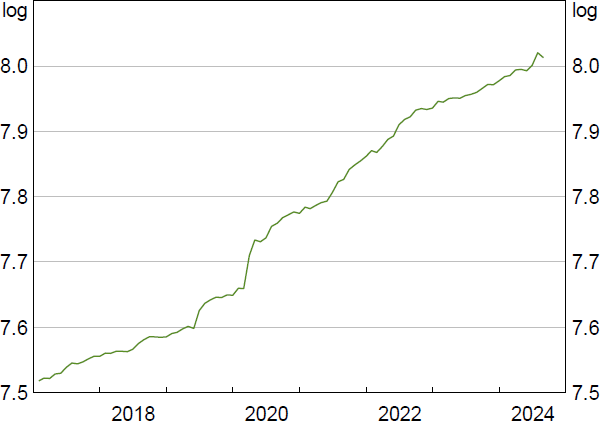
Source: APRA.
The usefulness of system deposits to capture growth in payments needs (i.e. transactional demand) likely varies over time. For example, credit growth creates deposits and is likely an indication of a growing economy or increased financialisation which increases payments needs. On the other hand, the central bank purchasing bonds from non-banks creates deposits but does not necessarily increase transactional demand if the proceeds from the bond sale solely represent an increase in household liquid wealth. During 2020, the stock of deposits rose while the daily average value of transactions settled fell (Figure 4). Since mid-2021, gross transaction volumes banks are required to manage have increased alongside deposit creation. The level of deposits also does not capture changes in the volatility of payment flows, which affects banks' transactional demand per dollar of deposits.
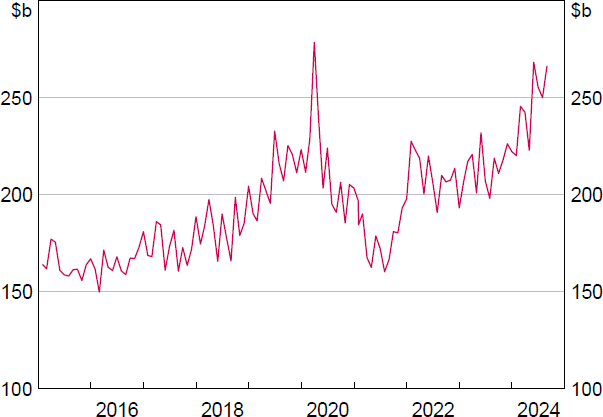
Source: RBA.
4.2 Precautionary demand
Banks might hold reserves as a precaution to protect against unexpectedly large outflows (Acharya and Rajan 2022). If facing an unexpectedly large withdrawal of funds, reserves are an immediate source of liquidity which can be drawn down. Other assets first need to be converted to reserves (‘monetised’) through outright sales or repo, which has the potential to increase the cost of meeting outflows by pushing down prices in outright markets or increasing repo rates.
Monetisation risk is often referenced in the context of liquidity coverage ratio (LCR) regulation. LCR banks are required to hold enough high-quality liquid assets (HQLA) to meet their anticipated net cash outflows (NCOs) if there was a liquidity stress event over the next 30 days. In Australia, reserves and bonds issued by federal, state and territory governments qualify as HQLA. While the LCR is agnostic on HQLA composition, banks may prefer to hold reserves to reduce monetisation risk as the size of outright and repo markets in which to liquidate HQLA securities in Australia is much smaller than banks' potential short-term liquidity needs (Figure 5). Operational considerations, such as settlement conventions (e.g. T + 2) and credit limits may also influence a bank's ability to monetise HQLA securities in size. The RBA's full-allotment OMO repo and other standing facilities could partially reduce precautionary demand for reserves because they allow counterparties to convert repo-eligible assets into reserves without limit.
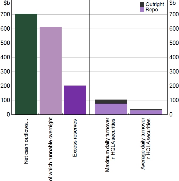
Note: Daily turnover in HQLA securities based on transactions settled in Austraclear between December 2021 and June 2024.
Sources: APRA; ASX; Author's calculations; RBA.
In 2023, the Australia Prudential Regulation Authority (APRA) consulted on targeted changes to strengthen liquidity management practices and crisis preparedness. In the review, APRA asked banks to begin formally assessing the monetisation risk of HQLA securities in their internal liquidity stress tests (APRA 2024). Similarly, regulators in the United States require banks to recognise the monetisation risk of HQLA securities. Banks, as a result, hold precautionary reserve balances to meet internal liquidity stress tests (Andolfatto and Ihrig 2019; Board of Governors of the Federal Reserve System 2019; Nelson 2022).
Like transactional demand, the precautionary demand curve is likely to be downward sloping, nonlinear and shifted by the stock of short-term runnable liabilities. A downward-sloping precautionary demand curve implies that additional reserves reduce monetisation risk by reducing the size of bonds which need to be monetised in a stress (or a lower probability of needing to monetise bonds at all) (Bush et al 2019). Eventually, there should be a ‘saturation point’ where reserve balances converge on the size of the largest possible outflow during a liquidity stress event such that additional reserves will no longer reduce monetisation risk. An increase in short-term liabilities increases the possible size of a liquidity stress event such that the marginal reserve balance becomes more valuable in reducing monetisation risk; short-term liabilities shift the precautionary demand curve. One potential omission from this framework is the effect of a change in banks' preference for how many precautionary reserves to hold per dollar of deposits. This preference could be driven by the distinction between reserves and government bonds in the eyes of regulators or a change in the composition of deposits from, say, insured to uninsured. My results are robust to using total or uninsured deposits.
Precautionary demand for reserves might have grown in recent years owing to an increase in the share of Australian banks' funding from short-term liabilities. As described above, unconventional monetary policy, alongside other factors, created a large amount of deposits – increasing banks' share of funding from short-term sources. More recently, the unwinding of unconventional policy measures has been accompanied by a modest fall in Australian banks' share of funding which is either overnight or at-call (Figure 6). The fall in claims on bank liquidity is unlike the US experience, where short-term claims on bank liquidity have not fallen during quantitative tightening (Acharya et al 2023). LCR banks' NCOs which they hold HQLA against are calculated by weighting each runnable liability proportional to the amount of funding which is expected to run in a 30-day liquidity stress event (known as a run-off rate). Weighting banks' overnight/at-call funding by their run-off rates shows that banks' anticipated overnight outflows in a stress have declined recently but remain elevated compared to pre-pandemic – potentially increasing banks' precautionary demand for reserves.
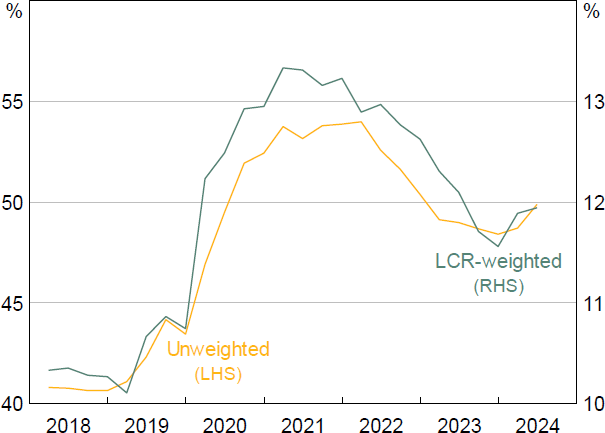
Sources: APRA; Author's calculations.
4.3 Relative value demand
Relative value demand represents reserves held to optimise banks' liquid asset portfolios (Borio, Disyatat and Schrimpf 2024). The LCR is agnostic on banks' HQLA portfolio composition, so banks should attempt to maximise profits by considering the risk-return trade-off between assets in the investable universe – reserves and government bonds. According to liaison, Australian banks consider the cost of holding reserves versus government bonds, where the return on these bonds is converted to a floating rate through swaps.[5]
If an LCR bank holds reserves, they receive a return equal to the ES rate. The five largest LCR banks receive an additional benefit as a result of the ‘major bank levy’ – a 6 basis point tax applied to select liabilities minus reserve holdings (Hawkins and Sanyal 2017). Banks subject to the bank levy pay 6 basis points less tax when holding reserve balances such that their opportunity cost of holding reserves is the ES rate plus 6 basis points (Equation (1)).
To compare the return on reserves with government bonds, LCR banks convert the bond's fixed rate of interest into an overnight, floating rate by first entering into an asset swap where they pay the bond's fixed rate of interest and receive the 3-month bank bill swap rate (BBSW) plus a spread. Then, LCR banks contract a basis swap to convert BBSW into the cash rate plus a spread. The return on the government bond comparable to reserves is equal to the cash rate plus the asset and basis swap spreads net of any capital costs (Equation (2)). Capital costs vary with the maturity of the government bond. If an LCR bank wants to close its position it would have to execute an asset swap in the opposite direction and take losses proportional with how far asset swap spreads have moved since the initial execution date. These losses are likely to be larger the longer the maturity of the swap contract.
From Equations (1) and (2), relative value demand is likely to be downward sloping as the spread between the cash rate and ES rate affects the trade-off between reserves and government bonds – as the cash rate declines relative to the ES rate it becomes more profitable for banks to hold reserves.[6] Relative value demand is likely shifted by changes in market prices which affect the trade-off between reserves and other HQLA (asset and basis swap spreads) (Borio 2023).
Prior to the pandemic, Australian Government Securities (AGS) were more profitable to hold than reserves (Figure 7).[7] During the pandemic, a decrease in the cash rate spread to the ES rate and a decrease in swap spreads meant holding reserves became a more attractive option to LCR banks. Since late 2022, swap spreads and the cash rate (relative to the ES rate) have risen – reducing the profitability of LCR banks' holding reserves.
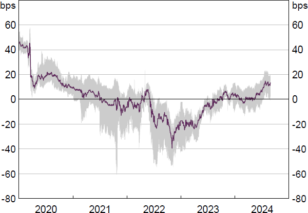
Notes: Excluding capital costs. Shaded area denotes the range of 1-, 2-, 3-, 5-, 7- and 10-year generic AGS.
Sources: Author's calculations; Bloomberg; RBA.
5. Data
The sample is from November 2020 to August 2024 – a period when reserves were in ample or excess supply. I chose this sample as there is potentially a structural break in reserve demand as a result of moving away from a scarce reserves system (Borio 2023). Between March and October 2020, the RBA conducted bond purchases which resulted in excess reserves rising from $3 billion to around $89 billion in March 2020 (Finlay, Titkov and Xiang 2022). Reserves then declined steadily to $37 billion by end October 2020. After the RBA announced $100 billion of bond purchases on 3 November 2020 the supply of reserves grew rapidly. The first observation is end November 2020.
5.1 Reserves
I use excess reserve balances in my estimation; balances held over and above any minimum reserve requirements imposed by the RBA. The RBA, in consultation with the Exchange Settlement Account holder, determines a minimum reserve requirement in proportion to the potential size of ‘after-hours’ payments to create a liquidity buffer. The minimum reserve requirement is set on an annual basis and must be maintained by banks at the close of business each day (RBA 2024b).
5.2 Overnight money market rates
I use overnight GC repo rates, rather than the (unsecured) cash rate, to estimate the demand for reserves. In the past, there was a convention by cash market participants to almost always conduct trades at the RBA's target rate (Kent 2024). While this convention is no longer in place, as evidenced by the cash rate trading below the RBA's target rate since the pandemic, many cash market participants still act as price-takers (Bristow and de Roure 2023). Price-takers will, by default, transact at the cash rate published each morning by the RBA which is based on yesterday's transactions (RBA 2022a). Since January 2022, only around 15 per cent of transactions took place at a rate different to the prevailing cash rate (Figure 8). The overnight GC repo market exhibits more price dispersion and a higher number of trades and volumes than the cash market (Bristow and Tang 2024).
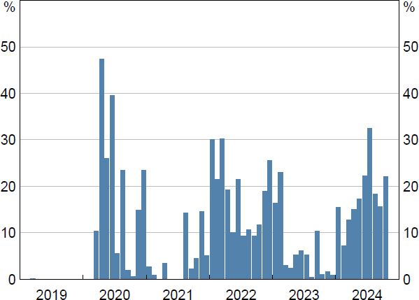
Sources: Author's calculations; RBA.
As of October 2024, Australia does not have an overnight GC repo benchmark rate. I construct a GC overnight repo rate using trade-level data submitted to APRA by ADIs and registered financial corporations in ARF 721.0A and a methodology consistent with repo benchmarks in other jurisdictions such as SOFR (Secured Overnight Financing Rate) and CORRA (Canadian Overnight Repo Rate Average) (Federal Reserve Bank of New York 2022; Bank of Canada 2020). For more details see Appendix A. Recently, the ASX have begun publishing an overnight GC repo rate – the Secured Overnight Funding Index Australia (SOFIA). SOFIA's usefulness for estimation is limited by the period over which it is published: January 2022 onwards. I compare my calculated overnight repo rate to SOFIA to check the validity of my rate calculation (Figure 9). The two series have a correlation coefficient of 0.83 and my empirical results are robust to the choice of repo rate (see Appendix B.3 for details).
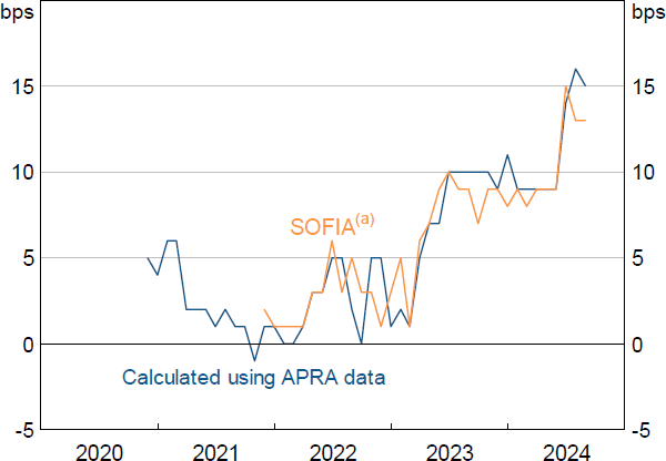
Note: (a) ASX's official beta estimate for SOFIA; volume-weighted median.
Sources: APRA; ASX; Author's calculations.
5.3 Deposits
For my measure of short-term liabilities, I use total ADI deposits as reported in APRA's monthly ADI statistics. Some reserve demand literature uses liquid deposits and other short-term claims on liquidity as they better represent liabilities which matter for banks' transactional and precautionary reserve demand (Acharya et al 2023). My empirical results are robust to a number of deposit measures including at-call deposits, uninsured deposits and total overnight/at-call liabilities.[8] I also test whether adding credit lines affects my results but they are statistically insignificant (see Appendix B.1 for details).
5.4 The cost of collateral
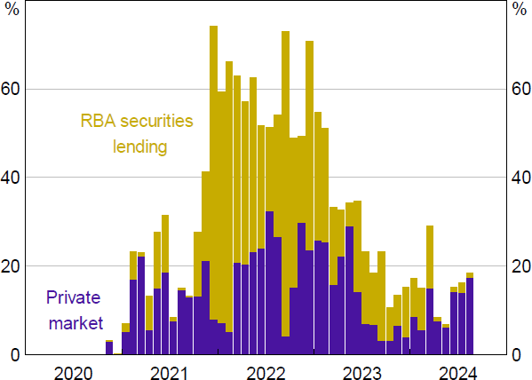
I account for the value of collateral when estimating reserve demand via the GC repo rate. Using ARF 721.0A data, I proxy for the value of collateral using the proportion of total GC overnight repo turnover which is trading 15 or more basis points below the GC repo rate (Figure 10). In calculating the measure, I include the value of bonds lent overnight through the RBA's securities lending facility – RBA counterparties can borrow government bonds under repo via this facility at a rate of 20 basis points below the ES rate. My results are robust to thresholds ranging from 5 to 15 basis points below the GC repo rate.
The large increase in securities lending by the RBA coincided with the RBA owning an increasingly large share of AGS. Market participants estimated that the ‘circulating’ free float of some individual bond lines available in circulation was as low as 10 per cent of the amount on issue (Aziz and Jackman 2022). Starting in early 2023, there has been a reduction in collateral scarcity and consequently a fall in RBA securities lending volume and a reduction in the number of bonds trading special in the repo market (Bristow and Tang 2024).
Sources: APRA; Author's calculations; RBA.
6 Model
6.1 Reserve demand
As in Lopez-Salido and Vissing-Jørgensen (2024), I model reserve demand as the benefit of holdings reserves:
In this framework, the demand curve is downward sloping as additional reserves increase convenience and relative value benefits, while reducing monetisation risks. As mentioned in Section 4, additional reserves have diminishing marginal benefit for managing a given stock of short-term liabilities or for holding against a liquidity stress event – making the demand curve nonlinear. An increase in deposits will shift the demand curve to the right as a result of increased transactional and precautionary demand.
Then, the profit-maximising condition for a bank borrowing via repo and investing in reserves sets the marginal cost of borrowing (repo rate plus the cost of giving up collateral) equal to the marginal benefit of investing in reserves (the ES rate plus the marginal benefit from holding reserves net of any balance sheet costs A):
Following Lopez-Salido and Vissing-Jørgensen (2024), I assume (Reserves, Deposits) net of balance sheet costs is log-linear in reserves and deposits as a base case:
Re-arranging Equation (4), including the assumption around the marginal benefit of holding reserves, I can express banks' reserve demand with respect to repo funding as:
An important determinant of repo rates is the balance of supply and demand for bonds financed under repo (the cost of the underlying collateral). If there are more cash lenders who want collateral than there are those who want to finance bonds under repo, GC repo rates tend to fall. For example, demand to accept German bunds as collateral leads GC repo rates collateralised by German bunds to be lower than GC repo rates collateralised by Italian or Spanish government bonds (Arrata et al 2020). On the other hand, repo rates can increase in response to bond issuance due to a corresponding increase in the demand to finance bonds under repo.
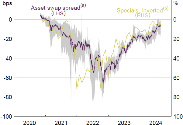
An appropriate measure of the cost of collateral should respond to changes in the supply of and demand for government bonds, but not be influenced by changes in the GC repo rate (relative to the ES rate) driven by other factors. On the face of it, asset swap spreads seem like an appropriate measure. Asset swap spreads are defined by the difference in the yield on government bonds and the expectation for BBSW over the life of the swap. Thus, shortages in the supply of government bonds that push down government bond yields are reflected by asset swap spreads moving lower. Asset swap spreads can also respond to increases in the GC repo rate driven by the demand to finance bonds under repo. This relationship is highlighted through the trade where market participants can pay the GC repo rate to fund a bond purchase and execute an asset swap – receiving a floating unsecured rate (BBSW) plus the asset spread. This means that asset swap spreads can respond to the expectation, over the life of the swap, for the difference between secured and unsecured rates, which could be rising due to increased demand for collateral.
However, through this mechanism, there is a possible endogeneity issue with using asset swap spreads if they respond to changes in repo rates caused by other factors. One measure which is highly correlated with asset swap spreads is the proportion of specials in the repo market (Figure 11). The advantage of using this measure is that rates on specials transactions are negotiated relative to the GC repo rate such that changes in the GC repo rate should not affect the proportion of bonds trading special. I proceed with this measure to proxy for the value of collateral posted under repo.
Notes:
(a) Shaded area denotes the asset swap spreads range of 1-, 2-, 3-, 5-, 7- and 10-year generic AGS.
(b) Proportion of repo volume trading 15 basis points below the GC repo rate; includes lending from the RBA securities lending facility.
Sources: APRA; Author's calculations; Bloomberg; RBA.
6.2 Reserve supply
Regressing the GC repo rate on the quantity of reserves only reveals the demand curve if all changes in the quantity of reserves represent shocks to supply. This is true if the quantity of reserves changes only for reasons other than responding to demand shocks or if the demand shocks that do change the quantity of reserves are controlled for in estimation. In the Australian context, a shock to demand for reserves could result in banks borrowing more from full-allotment OMO repo, which increases the quantity of reserves. The RBA balance sheet identity shows that reserves can be driven by changes in full-allotment OMO repo as well as ‘exogenous factors’, including changes to other central bank assets and liabilities.[9]
other assets and other liabilities are plausibly exogenous to the demand for reserves – making it a valid instrument to use in estimation. The main assets on the RBA's balance sheet during the sample period are bonds bought through unconventional monetary policy, TFF loans and the foreign exchange portfolio. Changes in these assets during the sample period have mostly been for monetary policy purposes and not heavily influenced by the demand for repo financing.
The main liabilities on the RBA's balance sheet during the sample period are government deposits, banknotes and other deposit accounts held predominately by foreign clients (e.g. other central banks). Movements in government deposits due to government spending, tax receipts, and bond issuance/maturities are likely independent of banks' reserve demand, once I control for the commercial bank deposits that these transactions create. In other words, the exclusion restriction would not hold if I excluded commercial bank deposits from the regression as the instrument would affect repo rates through a variable not controlled for. Deposit accounts held by foreign clients might respond to shifts in reserve demand. For example, a positive reserve demand shock leading to higher repo rates could incentivise foreign clients at the RBA to withdraw deposits and invest in repo – increasing the quantity of reserves. Foreign deposits declined substantially from around $26 billion in November 2021 to around $5 billion in June 2022. Since June 2022, these balances have been relatively small and stable. I include foreign deposits in my instrument to account for any potential endogeneity.
Taken together, other assets and other liabilities (besides foreign deposits) on the RBA balance sheet are broadly unaffected by shocks to reserve demand but highly correlated with reserves. Through the balance sheet identity, reserves minus full-allotment OMO and foreign deposits makes a valid instrument to use in estimation.
7 Results
I estimate reserve demand using the following equation:
where the repo rate is measured in basis points, is an error term and remaining parameters are to be estimated. The estimation is done using an instrumental variable (IV) approach using ln(Reserves – OMO Repo + foreign deposits) as an instrument for the log of reserves in the first stage. The first stage has an adjusted R-squared of 0.99 and its F-statistic is significantly greater than 10 – suggesting a strong instrument. Table 1 presents results for Equation (9) as a build – column 1 shows the estimation when only reserves are included in the regression, then deposits and the indicator of collateral cost are added. Column 4 shows the regression output when estimated using OLS.
The estimated coefficients have expected signs. The coefficient on reserves implies that a doubling in the supply of reserves results in repo rates decreasing by approximately 5 basis points. The coefficient on deposits indicates that for a 10 per cent increase in deposits, repo rates increase by approximately 4 basis points. The inclusion of deposits increases the adjusted R-squared substantively.
| Reserves only | Reserves and deposits | Full model – IV | Full model – OLS | |
|---|---|---|---|---|
| Constant | 19.04 (13.32) |
−400.50*** (36.52) |
−377.30*** (32.18) |
−379.20*** (31.34) |
| ln(Reserves) | −2.40 (2.01 |
−6.33*** (0.86) |
−4.78*** (0.99) |
−4.91*** (0.97) |
| ln(Deposits) | 55.91*** (4.72) |
52.01*** (4.32) |
52.33*** (4.17) |
|
| Specials | −0.05** (0.02) |
−0.05** (0.02) |
||
| Observations | 46 | 46 | 46 | 46 |
| AIC | 266.8 | 196.1 | 190.5 | 190.5 |
| Adjusted R2 | 0.04 | 0.80 | 0.82 | 0.82 |
| Estimation | IV | IV | IV | OLS |
| Notes: *, ** and *** denote statistical significance at the 1, 5 and 10 per cent levels, respectively. HAC standard errors in parentheses. | ||||
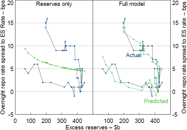
The simple model of reserve demand (Reserves only, Table 1) cannot explain the recent rise in repo rates (Figure 12, left panel). In contrast, the model including deposits and collateral cost (Full model – IV, Table 1) is able to explain the recent rise in repo rates (Figure 12, right panel). This suggests the demand curve for reserves has shifted to the right and that the shift can be explained by an increase in deposits.
Including the cost of collateral materially improves model fit and passes the log likelihood test at a 1 per cent significance level. The coefficient on specials indicates that repo rates tend to decline when there is a decline in the supply of collateral – a 10 percentage point increase in repo volume which is special is associated with GC repo rates declining by 0.5 basis points. These estimates imply the cost of collateral was worth 4 basis points at its peak (Figure 13). Before the end of 2021 and in the most recent period, where collateral has not been in short supply, the value of collateral has been small – mostly less than 1 basis point. This contrasts with Lopez-Salido and Vissing-Jørgensen (2024) who estimate non-time-varying collateral dynamics to be worth approximately 3 basis points in the US repo market.
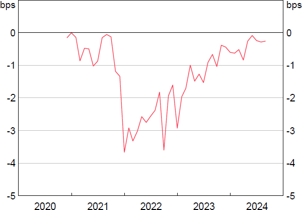
The inclusion of collateral cost decreases the coefficient on reserves (in absolute). A large part of the increase in reserves over the period was driven by the RBA's bond purchases which, in addition to increasing reserves, reduced the quantity of collateral available to the market – increasing the cost of collateral. When collateral cost is not accounted for in the regression, the coefficient on reserves is likely biased upward (in absolute) as it includes the effect of collateral cost on repo rates.
The difference in coefficients estimated using IV and OLS are small because the amount of full-allotment OMO repo and foreign client deposit movements over the estimation period has been relatively low and stable compared to the level of reserves. In other words, the sample period contains few shocks to demand which influence the quantity of reserves. Despite this, I prefer the IV estimates over OLS despite their slightly weaker precision, as even a small bias in the slope of the demand curve can have large impacts on the level of reserves which I qualify as ‘ample’.
8. Discussion
Holding deposits and the opportunity cost of collateral constant at their August 2024 level, I can plot the August 2024 reserve demand curve using Equation (10).
By Equation (10), banks' estimated demand is between $100 billion and $200 billion of excess reserves if private repo trades in line with the RBA's current OMO repo price (Figure 14). These estimates suggest banks should begin demanding additional funding from OMO repo when the level of reserves reaches between $100 billion and $200 billion in reserves. These estimates of reserve demand are significantly higher than the $3 billion in excess reserves required to implement monetary policy prior to the COVID-19 pandemic. Partly, what appears likely to be an increase in Australian banks' reserve demand reflects a decrease in the cost of borrowing under OMO repo – a run along banks' reserve demand curve. Though, a large part of the increase in reserve demand is the result of a shift in banks' demand curve explained by additional deposits.
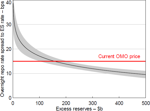
Note: Shaded area denotes 90 per cent confidence interval.
To demonstrate the shift in banks' reserve demand curve, I plot the August 2024 demand curve against the curve estimated using deposits and the cost of collateral as at November 2020. Figure 15 shows the shift in banks' demand up and to the right alongside more deposits.
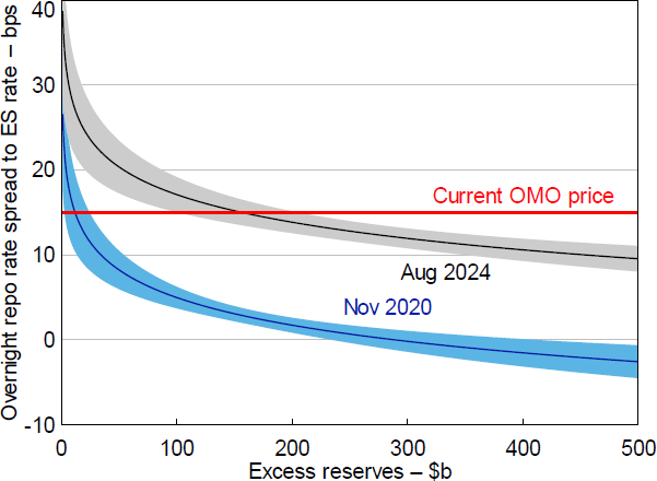
Note: Shaded areas denote 90 per cent confidence intervals.
Reserve demand estimates help inform when the RBA may transition from an excess reserves environment to its chosen system of ample reserves. To project the supply of reserves, one must consider the maturity profile of RBA bond holdings and other factors that influence reserves, such as changes in government and foreign deposits as well as growth in banknotes on issue. Using a projection of reserve supply, August 2024 reserve demand estimates suggest the RBA might be close to transitioning to its new ample reserves system – with the supply of reserves having dipped slightly below the upper 90 per cent confidence interval in the recent past (Figure 16). Taking the lower bound of the 90 per cent confidence interval, the RBA might transition to its new system as late as 2027.
The timing of this transition is subject to uncertainty associated with the future supply of and demand for reserves. For example, projecting supply requires assumptions around the level of government (and other) deposits and the growth in banknotes on issue, which are uncertain. On the demand side, the timing of the transition to ample reserves assumes no change in banking system deposits in the future and no change in banks' preference for how many precautionary reserves to hold per dollar of deposits. While RBA bond maturities will reduce the stock of deposits, there are other factors such as credit growth and banks purchasing additional HQLA securities to replace reserves lost when RBA bond holdings roll off which will likely mean deposits increase from their August 2024 level. An additional source of uncertainty relates to where overnight repo rates will trade relative to the RBA's OMO repo rate (ES rate + 15 basis points) in the ample reserves system. For simplicity, I have assumed repo rates trade at the same rate as the RBA's OMO repo. This might not be true as OMO repo is not a perfect substitute for overnight repo borrowing. It currently provides counterparties with 28-day repo funding, once a week, against a wide range of eligible collateral – including bank bonds, asset-backed securities and corporate bonds. How these design features affect where the reserve demand curve crosses the OMO price is not contemplated in my analysis.
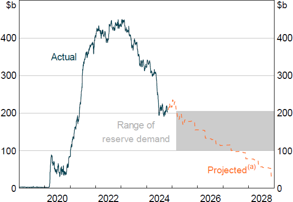
Note: (a) Assumes RBA bond holdings are held to maturity and no net change in RBA liquidity operations.
Sources: Author's calculations; RBA.
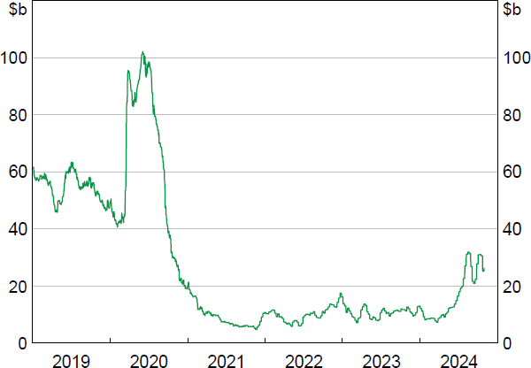
Despite these sources of uncertainty, the recent increase in bids at the RBA's OMO repo might suggest the reserve demand estimates presented in this paper are reasonable. In August 2024, the value of OMO repo outstanding grew to $32 billion – well above its $11 billion average since November 2020 despite excess reserves above $200 billion (Figure 17). Alternatively, liaison contacts noted the increase in OMO demand could have been driven by an increase in the cost of borrowing Australian dollars in the FX swap market. The increases in OMO volumes were also exacerbated by collateral and balance sheet limits binding on some repo market participants (RBA 2024a).
Reserve demand estimates presented in this paper are corroborated by those collated by staff in a survey following the RBA's future monetary policy implementation system consultation. Staff asked the following question to several large bank Treasury desks: ‘Please provide an estimate of the quantity of reserves your institution … expect[s] to hold in total based on current access to liquidity from the market and RBA’. Not all banks with active Exchange Settlement Accounts at the RBA were surveyed so the respondents' estimates were scaled up based on their share of system reserves as of June 2024. In this simple survey, banks indicated they intend to hold between $90 and $185 billion in reserves.
Source: RBA.
While estimates of reserve demand are inherently uncertain, the hypothesis that reserve demand has increased due to more deposits is relatively robust. This result holds across a variety of measures for short-term liabilities, including: total deposits, at-call deposits, uninsured deposits and total overnight/at-call funding. I opt to exclude credit lines and other off-balance sheet claims on banks' liquidity which could contribute to reserve demand as they are reported quarterly in Australia – reducing the number of observations in the sample to 15. When these claims are added to the regression framework, their coefficient sign (but not their statistical significance) supports the hypothesis that they contribute to reserve demand. Further work could be done to understand the link between these claims and banks' reserve demand. My results are robust to different measures of the cost of collateral (specials, bond–OIS spreads) and different sources for repo rates (APRA, ASX SOFIA) – see Appendices B.2 and B.3 for details.
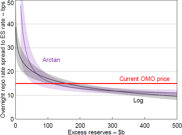
Despite the exact form of nonlinearity in the demand curve being unknown, deposits affect banks' reserve demand across a number of specifications, including: reserves entering in logs, an inverse relationship and arctangent functional forms (see Appendix B.4 for details). While my results are robust to functional form assumptions, different functional forms can lead to materially different outcomes for what level of reserves constitutes ample. For example, assuming an arctangent relationship between repo rates and the level of reserves results in a lower level of ample reserves but reserve demand becoming inelastic at much higher levels of excess reserves (Figure 18).
Note: Shaded areas denote 90 per cent confidence intervals.
Another limitation of this paper is that I do not account for the uneven distribution of reserves among banks. An uneven distribution of reserves amplifies the risk of spikes in money market rates if the banks holding most reserves are unwilling to lend them in the market. Copeland, Duffie and Yang (2021) outline that the September 2019 repo crunch in the United States was partly explained by reserve hoarding at large bank holding companies, who quoted high repo prices to counterparties seeking to borrow. This arguably caused a temporary loss of monetary control until the Federal Reserve stepped in to lend reserves via their OMO. Afonso et al (2020) argue that frictions in the interbank market may have prevented the efficient reallocation of reserves from institutions with sufficient balances to those who had balances below desired levels. They also find that some large dealers likely experienced an increase in intermediation costs which led them to charge higher spreads to cash borrowers in repo.
While this paper argues that deposits matter for reserve demand, it remains unclear whether higher deposits are the result of supply or demand factors. Have banks become more willing to supply short-term liabilities since the pandemic in response to a greater supply of reserves or has there been an increase in demand from households and businesses for liquid assets provided by banks? An emerging literature suggests banks may desire a shorter-dated funding mix permanently after a period of excess reserves supplied through unconventional monetary policy (Acharya and Rajan 2022; Acharya et al 2023). Future work could be done to investigate whether this finding applies in the Australian context.
Appendix A: Repo Rate Calculation
Institutions regulated by APRA who have gross repo and securities lending positions of greater than or equal to $1 billion are required to report their trades outstanding as at the end of the month. ARF 721.0A contains a subset of these repo dealers who, as part of this reporting requirement, submit trade-level data. Before calculating the rate, I apply a number of filters to these data.
First, I include only trades where general collateral 1[10] is posted. By market convention, these security types are able to be used interchangeably by market participants (AFMA 2023). Second, trades reported in ARF 721.0A only contain their residual (and not original) maturity. I filter the dataset to include only trades with an overnight residual maturity that were originated within the month. For example, I exclude trades originated in the month prior which have since decayed to have overnight residual maturity. I also remove all repo trades with the RBA. Finally, to remove bonds trading ‘special’, I order transactions based on their repo rate and remove the bottom 25 per cent of volume from the sample. From the remaining repo trades, I calculate the overnight GC repo rate as the volume-weighted median rate.
Appendix B: Robustness Tests
B.1 Alternative measures for deposits
| Total deposits | At-call deposits | Total overnight/at-call funding | Uninsured deposits | Credit lines | |
|---|---|---|---|---|---|
| Constant | −377.30*** (32.18) |
−561.50*** (65.21) |
−667.70*** (79.42) |
−289.10*** (24.89) |
−394.10*** (99.07) |
| ln(Reserves) | −4.78*** (0.99) |
−6.11*** (1.77) |
−4.57* (2.37) |
−4.81*** (1.07) |
−3.76** (1.69) |
| Specials | −0.05** (0.02) |
−0.10*** (0.03) |
−0.13** (0.04) |
−0.07*** (0.02) |
−0.06 (0.04) |
| ln(Deposits) | 52.01*** (4.32) |
52.61* (26.29) |
|||
| ln(At-call deposits) | 79.08*** (9.44) |
||||
| ln(Total overnight/at-call funding) | 90.22*** (11.27) |
||||
| ln(Uninsured deposits) | 43.57*** (3.59) |
||||
| ln(credit lines) | 1.34 (24.00) |
||||
| Observations | 46 | 46 | 15 | 46 | 15 |
| AIC | 190.5 | 209.7 | 74.5 | 193.4 | 69.5 |
| Adjusted R2 | 0.82 | 0.73 | 0.69 | 0.81 | 0.78 |
| Estimation | IV | IV | IV | IV | IV |
| Notes: *, ** and *** denote statistical significance at the 1, 5 and 10 per cent levels, respectively. HAC standard errors in parentheses. | |||||
B.2 Alternative measures for opportunity cost of collateral
| 3-year bond–OIS | 10-year bond–OIS | Asset swap spread | |
|---|---|---|---|
| Constant | −379.00*** (34.56) |
−453.60*** (39.88) |
−424.90*** (37.43) |
| ln(Reserves) | −4.62*** (1.01) |
−5.37*** (0.83) |
−5.51*** (0.97) |
| ln(Deposits) | 52.14*** (4.67) |
61.99*** (5.08) |
58.56*** (4.77) |
| 3-year bond–OIS | 6.56** (3.13) |
||
| 10-year bond–OIS | 6.13** (2.71) |
||
| Asset swap spread(a) | 0.07* (0.27) |
||
| Observations | 46 | 46 | 46 |
| AIC | 192.8 | 192.8 | 192.1 |
| Adjusted R2 | 0.82 | 0.82 | 0.82 |
| Estimation | IV | IV | IV |
|
Notes: *, ** and *** denote statistical significance at the 1, 5 and 10 per cent levels, respectively. HAC standard errors in parentheses. (a) Average of 1-, 3-, 5- and 10-year tenors. |
|||
B.3 Alternative sources for overnight GC repo rate
| SOFIA(a) | Calculated using APRA data | |
|---|---|---|
| Constant | −236.40*** (69.45) |
−377.30*** (32.18) |
| ln(Reserves) | −6.66*** (2.07) |
−4.78*** (0.99) |
| Specials | 35.60*** (7.07) |
52.01*** (4.32) |
| ln(Deposits) | −0.04** (0.02) |
−0.05** (0.02) |
| Observations | 34 | 46 |
| AIC | 135.6 | 190.5 |
| Adjusted R2 | 0.82 | 0.82 |
| Estimation | IV | IV |
|
Notes: *, ** and *** denote statistical significance at the 1, 5 and 10 per cent levels, respectively. HAC standard errors in parentheses. (a) ASX's official beta estimate for SOFIA; volume-weighted median. |
||
B.4 Alternative functional forms
| Inverse | Arctangent | Log | |
|---|---|---|---|
| Constant | −388.40*** (37.06) |
577.20** (275.90) |
−377.30*** (32.18) |
| 1/(Reserves) | 614.70*** (184.40) |
||
| Arctan (Reserves) | −614.70*** (184.40) |
||
| ln(Reserves) | −4.78*** (0.99) |
||
| Specials | −0.07*** (0.02) |
−0.07*** (0.02) |
−0.05** (0.02) |
| ln(Deposits) | 49.74*** (4.64) |
49.74*** (4.64) |
52.01*** (4.31) |
| Observations | 46 | 46 | 46 |
| AIC | 201.3 | 201.3 | 190.5 |
| Adjusted R2 | 0.78 | 0.78 | 0.82 |
| Estimation | OLS | OLS | OLS |
| Notes: *, ** and *** denote statistical significance at the 1, 5 and 10 per cent levels, respectively. HAC standard errors in parentheses. | |||
References
Åberg P, M Corsi, V Grossman-Wirth, T Hudepohl, Y Mudde, T Rosolin, F Schobert (2021), ‘Demand for Central Bank Reserves and Monetary Policy Implementation Frameworks: The Case of the Eurosystem’, European Central Bank Occasional Paper Series No 282.
Acharya VV, RS Chauhan, R Rajan and S Steffen (2023), ‘Liquidity Dependence and the Waxing and Waning of Central Bank Balance Sheets’, NBER Working Paper No 31050.
Acharya VV and R Rajan (2022), ‘Liquidity, Liquidity Everywhere, Not a Drop to Use – Why Flooding Banks with Central Bank Reserves May Not Expand Liquidity’, NBER Working Paper No 29680, rev November 2022.
AFMA (The Australian Financial Markets Association) (2023), ‘Reciprocal Purchase Agreements Conventions’, July. Available at <https://afma.com.au/getattachment/Standards/Market-Conventions/Sections/Content/Reciprocal-Purchase-Agreements-Conventions-2023-07.pdf?lang=en-AU>.
Afonso G, M Cipriani, A Copeland, A Kovner, G La Spada and A Martin (2020), ‘The Market Events of Mid-September 2019’, Federal Reserve Bank of New York Staff Report No 918.
Afonso G, D Giannone, G La Spada and JC Williams (2022), ‘Scarce, Abundant, or Ample? A Time-varying Model of the Reserve Demand Curve’, Federal Reserve Bank of New York Staff Report No 1019, rev April 2024.
Afonso G, D Giannone, G La Spada and JC Williams (2024), ‘When Are Central Bank Reserves Ample?’, Federal Reserve Bank of New York Liberty Street Economics blog, 13 August, viewed 9 September 2024. Available at <https://libertystreeteconomics.newyorkfed.org/2024/08/when-are-central-bank-reserves-ample/>.
Andolfatto D and JE Ihrig (2019), ‘The Fed and a Standing Repo Facility: A Follow-up’, Federal Reserve Bank of St. Louis On the Economy blog, 19 April, viewed 10 September 2024. Available at <https://www.stlouisfed.org/on-the-economy/2019/april/fed-standing-repo-facility-follow-up>.
APRA (Australian Prudential Regulation Authority) (2024), ‘APRA Finalises Targeted Changes to Strengthen Banks' Liquidity and Capital Requirements’, Media Release, 24 July.
Arrata W, B Nguyen, I Rahmouni-Rousseau and M Vari (2020), ‘The Scarcity Effect of QE on Repo Rates: Evidence from the Euro Area’, Journal of Financial Economics, 137(3), pp 837–856.
Aziz A and B Jackman (2022), ‘The RBA and AOFM Securities Lending Facilities’, RBA Bulletin, December.
Bank of Canada (2020), ‘Methodology for Calculating the Canadian Overnight Repo Rate Average (CORRA)’, 15 June, viewed 14 November 2024. Available at <https://www.bankofcanada.ca/rates/interest-rates/corra/methodology-calculating-corra/>.
Bech ML, A Martin and J McAndrews (2012), ‘How the High Level of Reserves Benefits the Payment System’, Federal Reserve Bank of New York Liberty Street Economics blog, 27 February, viewed 23 September 2024. Available at <https://libertystreeteconomics.newyorkfed.org/2012/02/how-the-high-level-of-reserves-benefits-the-payment-system/>.
Board of Governors of the Federal Reserve System (2019), ‘August 2019 Senior Financial Officer Survey’.
Borio C (2023), ‘Getting up from the Floor’, BIS Working Paper No 1100.
Borio C, P Disyatat and A Schrimpf (2024), ‘The Double-faced Demand for Bank Reserves and its Implications’, VoxEU Column, 15 February, viewed 24 September 2024. Available at <https://cepr.org/voxeu/columns/double-faced-demand-bank-reserves-and-its-implications>.
Bräuning F (2018), ‘The Liquidity Effect of the Federal Reserve's Balance Sheet Reduction on Short-term Interest Rates’, Federal Reserve Bank of Boston, Currency Policy Perspectives No 18-1.
Bristow L and C de Roure (2023), ‘Recent Developments in the Cash Market’, RBA Bulletin, June.
Bristow L and M Tang (2024), ‘The Australian Repo Market: A Short History and Recent Evolution’, RBA Bulletin, July.
Bulusu N, M McNeely, K McRae and J Witmer (2023), ‘Estimating the Appropriate Quantity of Settlement Balances in a Floor System’, Bank of Canada Staff Discussion Paper 2023-26.
Bush R, A Kirk, A Martin, P Weed and P Zobel (2019), ‘Stressed Outflows and the Supply of Central Bank Reserves’, Federal Reserve Bank of New York Liberty Street Economics blog, 20 February, viewed 24 September 2024. Available at <https://libertystreeteconomics.newyorkfed.org/2019/02/stressed-outflows-and-the-supply-of-central-bank-reserves/>.
Chen Z, N Kourentzes and RM Veyrune (2023), ‘Modeling the Reserve Demand to Facilitate Central Bank Operations’, IMF Working Paper No WP/23/179.
Cheung B and S Printant (2019), ‘Australian Money Market Divergence: Arbitrage Opportunity or Illusion?’, RBA Research Discussion Paper No 2019-09.
Copeland A, D Duffie and Y Yang (2021), ‘Reserves Were Not so Ample after All’, Federal Reserve Bank of New York Staff Report No 974, revised July 2024.
Debelle G (2021), ‘Monetary Policy during COVID’, Shann Memorial Lecture, Online, 6 May.
Federal Reserve Bank of New York (2022), ‘Calculation Methodology for the SOFR Averages and Index’, Additional Information about Reference Rates Administered by the New York Fed, 24 January, viewed 14 November 2024. Available at <https://www.newyorkfed.org/markets/reference-rates/additional-information-about-reference-rates#tgcr_bgcr_sofr_calculation_methodology>.
Finlay R, D Titkov and M Xiang (2022), ‘The Yield and Market Function Effects of the Reserve Bank of Australia's Bond Purchases’, Economic Record, 99(326), pp 359–384.
Frost PA (1971), ‘Banks’ Demand for Excess Reserves', Journal of Political Economy, 79(4), pp 805–825.
Hauser A (2023), ‘“Less is More” or “Less is a Bore”? Re-calibrating the Role of Central Bank Reserves', Keynote speech given at the annual Kings College London Bank of England Watchers’ Conference, London, 3 November.
Hawkins P and K Sanyal (2017), ‘A Levy on Major Banks and Improving Accountability for Bank Executives’, in ‘Budget Review 2017–18’, Parliamentary Library Research Paper Series, 2016–17, 19 May, pp 30–31.
Johnson C (2022), ‘Trends in Australian Banks' Bond Issuance’, RBA Bulletin, September.
Kent C (2024), ‘The Future System for Monetary Policy Implementation’, Speech at the Bloomberg Australia Briefing, Sydney, 2 April.
Kopec K and C Rao (2022), ‘The Evolution of Interbank Settlement in Australia’, RBA Bulletin, March.
Lopez-Salido D and A Vissing-Jørgensen (2024), ‘Reserve Demand, Interest Rate Control and Quantitative Tightening’, Unpublished manuscript, Federal Reserve Board, 25 July.
Meinecke F (2023), ‘What Do We Know about the Demand for Bank of England Reserves?’, Bank of England Bank Overground blog, 22 February, viewed 11 September 2024. Available at <https://www.bankofengland.co.uk/bank-overground/2023/what-do-we-know-about-the-demand-for-bank-of-england-reserves>.
Nelson B (2022), ‘Bank Examiner Preferences Are Obstructing Monetary Policy’, Bank Policy Institute, Bank Liquidity blog post, 19 September, viewed 25 September 2024. Available at <https://bpi.com/bank-examiner-preferences-are-obstructing-monetary-policy/>.
Nicolae L (2020), ‘The Effects of Liquidity Regulation on Bank Demand for Reserves and the Federal Reserve's Balance Sheet Policy’, Harvard Kennedy School, Mossavar-Rahmani Center for Business and Government, M-RCBG Associate Working Paper Series No 140.
Ramsden D (2018), ‘Finding the Right Balance’, Speech given at the Society of Professional Economists Annual Conference ‘The Global Outlook: Better Growth, Bigger Risks’, London, 28 September.
RBA (Reserve Bank of Australia) (2020), ‘Box D: Recent Growth in the Money Supply and Deposits’, Statement on Monetary Policy, August.
RBA (2022a), ‘Cash Rate Procedures Manual’, Monetary Operations resource, updated 19 December.
RBA (2022b), ‘Review of the Bond Purchase Program’, Reserve Bank Board Review, September.
RBA (2024a), ‘Chapter 1: Financial Conditions’, Statement on Monetary Policy, May.
RBA (2024b), ‘Liquidity Facilities’, Domestic Market Operations and Liquidity Facilities Technical Note, updated 16 July.
Reis R (2016), ‘Funding Quantitative Easing to Target Inflation’, Centre for Macroeconomics Discussion Paper No CFM-DP2016-26.
Schnabel I (2024), ‘The Eurosystem's Operational Framework’, Speech given at the Money Market Contact Group meeting, Frankfurt am Main, 14 March.
Smith AL (2021), ‘Do Changes in Reserve Balances Still Influence the Federal Funds Rate?’, Federal Reserve Bank of Kansas City Economic Review, First Quarter, pp 5–34.
Smith AL and VJ Valcarcel (2023), ‘The Financial Market Effects of Unwinding the Federal Reserve's Balance Sheet’, Journal of Economic Dynamics and Control, 146, Article 104582.
Sveriges Riksbank (2019), ‘The Riksbank's New Operational Framework for the Implementation of Monetary Policy’, Consultation document, July.
Veyrune R, G della Valle and S Guo (2018), ‘Relationship between Short-term Interest Rates and Excess Reserves: A Logistic Approach’, IMF Working Paper No WP/18/80.
Vissing-Jørgensen A (2023), ‘Balance Sheet Policy above the ELB’, Paper presented at the ECB Forum on Central Banking 2023 ‘Macroeconomic Stabilisation in a Volatile Inflation Environment’, Sintra, 26–28 June.
Acknowledgements
I would like to thank Bill Nelson, Dmitry Titkov, Richard Finlay, Anthony Brassil, Duke Cole, Gian-piero Lovicu, David Jacobs, Christopher Kent, Sean Dowling, Matthew Read, Jeremy Gehrig, Fabio Rustia, Jon Cheshire, Callum Ryan and participants in internal Reserve Bank seminars for helpful comments and suggestions. The views expressed in this paper are my own and do not necessarily reflect the view of the Reserve Bank of Australia. I am solely responsible for any errors.
Footnotes
Unless stated otherwise, I use ‘reserves’ to refer to excess reserves. For more details, see Section 5.1. [1]
Considering the maturity profile of RBA bond holdings and other factors that drain reserves, such as growth in banknote demand. See Section 8 for more detail. [2]
There is some evidence that additional reserves led to faster settlement of payments in the United States (Bech, Martin and McAndrews 2012). Payment efficiency has also increased in Australia, albeit to a lesser extent than the United States, since operating with a higher level of reserves (Kopec and Rao 2022). [3]
There may still be some cost associated with encumbering collateral intraday or an operational cost related to using the facility. [4]
Some banks consider the cost of hedging using futures, though this is less common. [5]
I use the repo rate, not the cash rate, to estimate demand for reserves. However, assuming negligible credit and liquidity risk difference between secured and unsecured rates, the spread between the repo and cash rate represents the value of collateral which I control for in my estimation. Thus, banks' reserve demand with respect to repo financing will also slope downward. [6]
I exclude showing hedged returns on state and territory government bonds for simplicity. [7]
I construct total overnight funding using APRA form ARF 210.3.2 and calculate credit lines by aggregating LCR banks' total committed facilities, other contractual obligations to extend funds and other contingent funding obligations from Tables 14, 15 and 16 in LCR banks' reporting form ARF 210.1A. [8]
Other liabilities include the RBA's capital position which is excluded here for simplicity. [9]
Australian Government and semi-government bonds, Treasury notes, and Australian Government and semi-government indexed bonds used as collateral. [10]