RDP 2024-10: How Do Global Shocks Affect Australia? 3. A Global FAVAR Model for Australia

We use a FAVAR model to quantify the importance of global shocks in driving variation in Australian variables and explore the channels through which they spill over. The FAVAR approach is particularly suited for this task. The main assumption of the approach is that a small number of unobserved factors drive common variation in a wide range of variables across countries (Stock and Watson 2016). Under this assumption, these factors then allow us to span the space of global shocks that drive most of the variation in the global economy in a data-driven way without having to restrict our analysis to shocks originating in a certain country, or specific shocks affecting only a small set of variables. Moreover, the model also provides the parsimony of a small-scale VAR in modelling the global economy, allowing us to study the responses of a wider range of Australian variables to these global shocks.

To illustrate a benefit of spanning the space of global shocks, imagine a bilateral VAR with the United States and Australia. First, this model should adequately capture global shocks affecting Australia that originate in or strongly affect the United States, but might miss shocks such as a financial crisis in Asia, which could impact Australia without having much effect on the United States. To the extent that an Asian financial crisis (as an example) is reflected in co-movement in global variables other than US variables, our global factors are more likely to capture this shock. Second, we also do not have to limit ourselves to a small set of US variables that we believe capture shocks of relevance to Australia. As the FAVAR can be informed by a large set of variables from each country, more sectors and a broad range of variables can be included, which can be particularly important if there is measurement or reporting error in variables.

However, the FAVAR approach also has drawbacks. As with most factor model approaches, the estimated factors are difficult to interpret, and this model is less suitable for identifying and estimating the effect of particular shocks, such as specific types of demand or supply shocks originating in a specific country. Additionally, the factor model approach, while in theory better able to span the space of global shocks, is effectively agnostic to the actual structure of the global economy and its relationship with Australia. The factors are appropriate for summarising the common variation in the global panel of variables, but this is not necessarily the variation that matters most for the Australian reality. For instance, imagine in the previous example that instead the United States actually is by far the most important foreign economy to Australia. In that case, abstracting away from US idiosyncratic shocks in order to capture global variation will reduce the extent to which the global shocks in the model can explain variation in Australian variables. We seek to address these concerns in Section 4 by comparing our FAVAR analysis to standard two-country VARs and by examining the explanatory content of all the estimated factors.

We estimate the FAVAR in two stages. First, we estimate the factors using principal components analysis (PCA) on the global data. Second, we then estimate the VAR using the global factors as our foreign block, and some observed Australian variables as our domestic block.

3.1 Estimating the factors

3.1.1 FAVAR model

For our FAVAR specification we draw on Bernanke et al's (2005) original model, and Mumtaz and Surico's (2009) extension to a small open economy. The FAVAR can be expressed in static form as an observation equation which specifies the factors, and a transition equation, which specifies the VAR.

Suppose the state of the global economy can be summarised by K unobserved factors, estimated over N foreign variables. The observation equation of this system is:

where F_t is a K×1 vector of factors and $X_t^F$ an N^F×1 vector of foreign variables with $K\ll N^F$. ${\Lambda }^F$ is an N^F×K matrix of factor loadings, while e_t is an N^F×1 vector of idiosyncratic, zero mean disturbances.

The joint dynamics of the global factors F_t and the Australian variables then evolve according to the transition equation:

where the Australian variables are the N×1 vector $X_t^A,\Phi \left(L\right)$ is a conformable lag polynomial of order p, and u_t is a vector of (serially uncorrelated) mean zero innovations. We select the lag order with Akaike information criterion. To operationalise the assumption that global factors do not respond to domestic variables, we restrict the coefficients within $\Phi \left(L\right)$ that let $X_{t-1}^A$ affect F_t to be zero.^[4]

We first estimate the factors using PCA, such that the factors are identified by the principal components normalisation (since the factors are in principle only identified up to a rotation) (Bai and Ng 2013; Stock and Watson 2016). That is, the columns of ${\Lambda }^F$ are by construction orthogonal and are scaled to have the unit norm ${\Lambda }^{F^{\prime }}{\Lambda }^F/N^F=I$ with F′F diagonal. ${\sum }_F=E\left(F_t{F^{\prime }}_t\right)$ is diagonal with weakly decreasing elements. Having extracted the factors, we then estimate the transition equation of the VAR using the global factors as our foreign block in a separate second step.^[5]

3.1.2 Data

We construct a global panel of variables related to activity, prices, interest rates, financial markets and commodities across nine advanced economies and four emerging economies: the United States, Japan, France, Germany, Italy, Korea, Canada, the United Kingdom, New Zealand, China, India, Mexico and Russia. These countries accounted for around 70 per cent of global GDP, around 65 per cent of Australia's two-way trade (Department of Foreign Affairs and Trade 2021b), and around 59 per cent of total investment in Australia in 2021 (Department of Foreign Affairs and Trade 2021a).^[6] In particular, for each country, we collected:

• Activity variables: levels of real GDP, real net exports, real final consumption, indices of real industrial production, and unemployment rates;
• Prices variables: indices of consumer prices, producer prices, import prices and GDP deflators;
• Interest rate variables: central bank policy rates, 90-day interbank rates and 10-year government bond yields;
• Financial variables: domestic stock market indices and exchange rates against the US dollar.

We also add several global or regional variables: WTI and Brent oil, sub-components of the RBA's Index of Commodity Prices, corporate bond spreads for the United States, Latin America, the euro area and emerging Asia, and volatility indices for some stock markets and for global currencies. As the FAVAR requires stationary variables, we transform the data as in Stock and Watson (2016). Variables measured in levels (such as the GDP indices) were transformed to log differences, while variables measured as rates (interest rates, unemployment rates, exchange rates and spreads) were transformed to differences.^[7] See Appendix A for a complete summary of the 189 series used and their transformations.

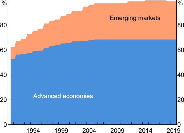
The foreign and global data were primarily collected from the St Louis Federal Reserve Economic Database (FRED) and the IMF International Financial Statistics (IFS) database. Variables that were missing from these sources were supplemented with data from Bloomberg, Reuters Refinitiv, CEIC and the Wind Financial Terminal. However, there are still some missing data, largely from series that only began to be published after 1990, with much of this being emerging market data (Figure 1). To estimate the factors using principal components, we fill in the missing data by applying Stock and Watson's (2002) expectations maximisation algorithm.

Data for the domestic Australian block were collected from the ABS or RBA statistical tables. The variables were gathered on a monthly or quarterly basis, as available, but we aggregate monthly variables to a quarterly frequency by taking their end-of-quarter levels to align the frequency of the available variables.^[8] Due to data availability, and due to concerns that the volatility of the COVID-19 pandemic will significantly affect the results, we estimate the FAVAR using quarterly data from 1990 to the end of 2019.^[9]

3.1.3 Description of the factors

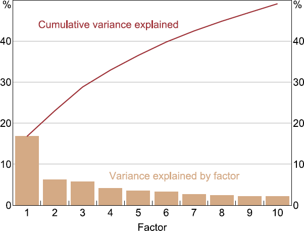
We estimate the factors using PCA on the panel of global data. Applying Bai and Ng's (2002) information criteria, we select three factors from the panel of foreign variables which cumulatively explain approximately 30 per cent of the variation in the data (Figure 2).^[10] The PCA factors are orthogonal by construction. These factors cannot be interpreted as particular ‘structural’ shocks to the global economy, but rather capture the sum of the common global shocks that explain the most variation in the global panel. This approach illustrates the distinction between ‘global’ and ‘foreign’ shocks. To the extent that the factors only capture information that best explains common variation across the whole panel, we do not investigate how foreign shocks affecting only one country or one sector (i.e. that do not drive variation in broader global economic or financial conditions) affect the Australian economy.

In turn, we assume that these factors have the highest potential to explain the variation in Australian domestic variables.^[11] While this prohibits us from assessing how any specific foreign shock affects the Australian economy, it allows us to assess how much of the variation in Australian data can be explained by common global shocks and through which channels they are transmitted to Australia.

In essence, our approach amounts to estimating how much the variation in the first several factors, which we assume adequately capture the relevant global shocks, explain variation in Australian economic and financial variables. We relax this assumption in Section 4.1.3 and explore whether other factors beyond the third factor drive a significant share of the variation in Australian data.

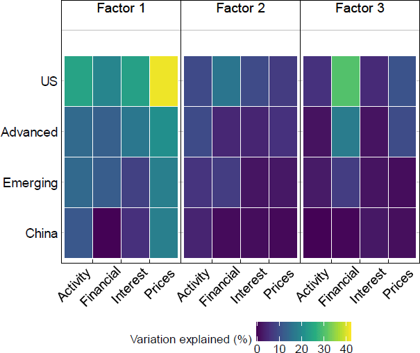
The first factor appears to explain substantial variation in categories of variables across the panel, especially for activity, interest rates and prices. The first factor has the strongest loading on US prices, explaining on average 41 per cent of variation for these variables (Figure 3 and Table B1). The third factor clearly explains more variation in financial variables than it does in other variables. The second factor is less clear, and it appears to loosely explain roughly equal variation in different types of variables, but seems to capture slightly more variation in US variables.

The first three factors together explain a particularly high proportion of variation in US variables, other advanced economy variables, and global variables, explaining 50 per cent, 29 per cent, and 35 per cent of the variation on average across the variables, respectively.^[12] The factors explain noticeably less variation in variables for non-China emerging markets, explaining 21 per cent of the variation on average, and even less for China, where the factors explain 12 per cent of the variation on average. This may raise concerns that we are missing important shocks originating in China, which we address in Section 4.1.4.

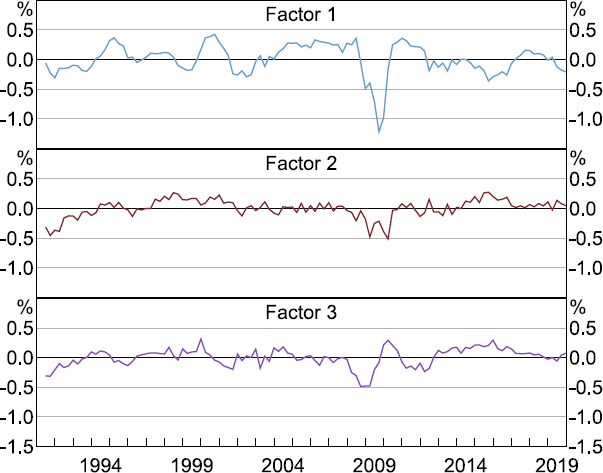
The first and third factor drop sharply during the GFC (Figure 4). This aligns with the interpretation of these factors as broadly relating to activity/prices and financial markets, respectively. The interpretation of the second factor is again less clear. While this may raise questions as to how to interpret these factors (a common issue in factor models), the specific interpretation of each factor is not particularly important as we do not attempt to use these factors to construct structural shocks for the purposes of the analysis in Section 4.

Footnotes

We include Australian variables directly in the FAVAR rather than modelling the Australian economy via a factor model of a large suite of Australian variables. This allows foreign factors to affect Australian variables directly, rather than only through their common variation with estimated domestic factors. [4]

FAVARs can also be estimated in a single stage using maximum likelihood methods, as in Hartigan and Wright (2021). We apply the two-stage approach for simplicity, as in most applications the two methods do not seem to produce significantly different results (Stock and Watson 2016). [5]

This likely underestimates the proportion of total investment from these countries, as some investment that originates in these countries may be recorded as originating from an intermediate country (such as a tax haven). [6]

The choice of transformations is supported by Dickey-Fuller tests. [7]

We used quarter-end to align the timing of monthly data with some quarterly data that is only available as quarter-ended. [8]

Our main results are robust to estimating the model starting from 1993 to align with the inflation-targeting period. [9]

The criterion determines the optimal number of factors based on the marginal added variation explained relative to a penalty term to ensure parsimony. Considering the range of sectors (real and financial) and different geographic regions in the global panel, the fact that three factors alone capture around 30 per cent of variation in the data suggests that the factors are indeed capturing important global information. [10]

For the main results of the paper, we estimate the factors freely across categories of variables (e.g. activity, prices) rather than estimating the factors within categories as in Mumtaz and Surico (2009). We choose this purely data-driven approach to estimating the factors to maximise the common variation in the global data explained by the factors and because we do not aim to identify particular types of foreign shocks. While restricting the estimation of factors as in Mumtaz and Surico (2009) could aid interpretation when paired with further identifying assumptions, the additional restriction of estimating factors for each category separately would reduce the common variation captured by the global factors under this approach. That said, our results are robust to estimating factors within blocks of categories. [11]

Global variables include global financial indices and globally traded commodities such as oil (see Appendix A). [12]