Bulletin – September 2018 Australian Economy The Cyclical Behaviour of Labour Force Participation
- Download 551KB

Abstract
When economic conditions improve, more people enter the labour force. Understanding the nature of this cyclical relationship between participation and economic activity is important for determining the amount of slack in the labour market and predicting how the economy will respond to changes in economic conditions. The participation rates of young people, 25–54-year-old females and older males are the most responsive to changes in economic conditions. If the participation rate did not adjust, expansions would be more inflationary, while recessions would be more disinflationary and lead to larger increases in involuntary unemployment.
Introduction
The labour force participation rate records the number of people in employment or looking for work as a share of the total working-age population. Over recent decades, the participation rate trended up and is currently a little under 66 per cent of the working-age population (Graph 1). Much of this rise reflects long-term behavioural shifts, such as the increasing tendency of women to stay in the labour force throughout their working lives and older workers to retire later.[1]
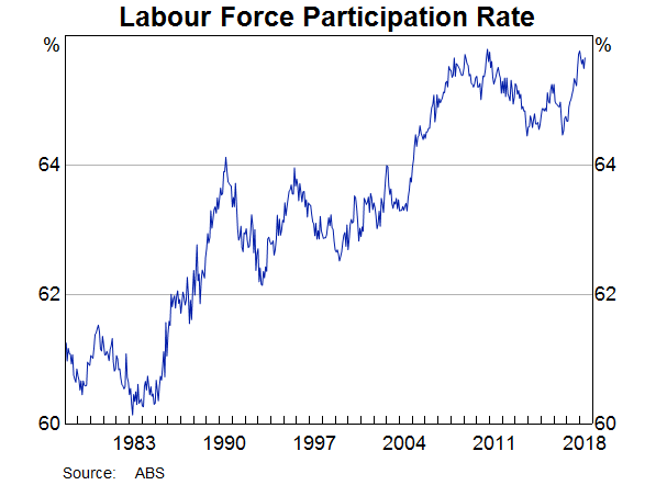
In the shorter run, the participation rate varies considerably around this long-run trend. Between 1990 and 1993 the participation rate fell by 1¾ percentage points as the economy entered recession. More recently, between late 2016 and the middle of 2018, a period of strong employment growth, the participation rate rose by 1 percentage point.
Short-run movements in the participation rate can occur for a number of reasons. Long-term behavioural shifts may not play out smoothly over time. There may be measurement error or ‘noise’ in the data. And the participation rate may have a cyclical component, reflecting a tendency for people to enter or leave the workforce as economic conditions and employment opportunities improve or deteriorate. Understanding this cyclical component – which can be thought of as the labour supply response to changes in the demand for labour – is important because it can help us to assess the amount of spare capacity in the labour market. The extent of spare capacity has implications for the outlook for wages growth and inflation as the labour market adjusts to shifts in demand.
This article explores the cyclical behaviour of the participation rate in three ways. First, we investigate whether the participation rate has a cyclical component at an aggregate level by identifying the relationship between short-run movements in the participation rate and the economic cycle. Second, we delve into the detailed labour force data to identify the groups in the labour force whose participation rates are the most sensitive to economic conditions, and consider whether this relationship has changed over time. Third, we use the RBA's macroeconomic model, MARTIN, to explore the macroeconomic consequences of cyclical variation in labour force participation.
We report three key findings. First, the participation rate has a large and economically meaningful cyclical component. At an annual frequency, around 40 per cent of a cyclical increase in employment is typically met by a rise in the labour force participation rate. Second, the cyclical sensitivity of labour force participation varies across the community, with young people, 25–54-year-old females and older males being the most likely groups to enter or leave the labour force in response to changes in economic conditions. Third, changes in the participation rate are an important shock absorber for the economy. Without them, booms would be more inflationary and downturns would be more disinflationary and lead to larger increases in involuntary unemployment.
Is There Evidence of a Cyclical Participation Rate at an Aggregate Level?
Our first set of results document the existence of a cyclical component of the participation rate at an aggregate level. To do so, we need to distinguish cyclical movements in the participation rate from structural ones. An increase in the participation rate is cyclical if stronger economic conditions encourage more people to enter or stay in the workforce. Structural increases in the participation rate relate to longer-term or supply-side factors, for example, if longer lifespans lead to an increase in the average age at which people retire. We investigate this question in two ways. First, we graph the relationship between the participation rate and other labour market variables over short horizons, over which cyclical factors are likely to account for a larger share of movement than structural factors. We then confirm these results in a more formal setting with the aid of a small model that uses statistical techniques to distinguish between cyclical and structural influences on the participation rate.
If cyclical factors matter, we would expect the participation rate to rise alongside an increase in employment over relatively short timeframes. The top panel of Graph 2 plots the relationship between year-ended changes in the participation rate and in the number of people in work expressed as a proportion of the total working-age population (the employment-to-population ratio) over the past four decades.[2] Each dot shows the relationship at a single point in time. The line shows the average relationship between the two series, determined by fitting a linear trend to the individual observations. Over the long run, we expect to see a positive relationship between the two series, as a structural increase in the share of the population in employment is likely to be accompanied by a rise in the participation rate.[3] While this effect would also be evident to a degree at an annual frequency, changes in economic conditions are likely to account for most changes in the employment-to-population ratio at this frequency. The fact that we observe a positive short-run relationship between the two series is consistent with at least some of the movement in the participation rate reflecting cyclical factors.
Another way to gauge the extent to which changes in the participation rate are cyclical is to examine the co-movement between the participation rate and the unemployment rate (middle panel of Graph 2). The persistent component of the unemployment rate – the Non-Accelerating Inflation Rate of Unemployment (NAIRU) – can be reasonably assumed to evolve slowly over time. Therefore most short-run movements in the unemployment rate reflect economic conditions – the unemployment rate tends to fall during economic expansions and rise during downturns. Because of this, movements in the participation rate that reflect cyclical factors will tend to have a negative relationship with the unemployment rate. In contrast, increases in the participation rate that reflect structural factors are likely to be associated with rises in the unemployment rate if it takes more time for new labour force entrants to find employment.
The participation rate moves less closely with the unemployment rate than it does with the employment-to-population ratio. But, on average, the relationship is negative. That is, at an annual frequency, cyclical forces appear to dominate and improvements in economic conditions that lead to falls in the unemployment rate are associated with rises in the participation rate.
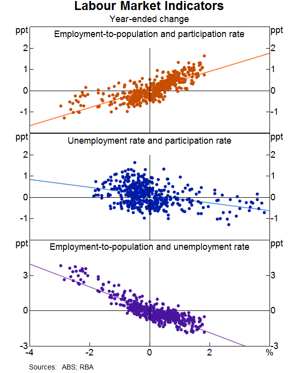
The relationships in the top two panels of Graph 2 are not mechanical. For example, over short horizons, changes in the employment-to-population ratio could, in principle, be met entirely by changes in the number of people who are unemployed, rather than by increases in participation. The bottom panel of Graph 2 shows that the relationship between changes in the unemployment rate and changes in the employment-to-population ratio is extremely close. Nonetheless, the unemployment rate typically does not move by enough to fully account for changes in the employment-to-population ratio.[4] Taking the regression lines from the three panels of Graph 2 together suggests that, on average, 40 per cent of a cyclical increase in the employment-to-population ratio will be met by an increase in the participation rate, with the remainder coming from a fall in the unemployment rate. This rule of thumb appears to have been remarkably stable over the past four decades, despite increasing labour market flexibility and a large decline in macroeconomic volatility over this period.
Using a statistical model to uncover the trend and cyclical components
The relationships in Graph 2 suggests that there is a cyclical component of the participation rate. We use a statistical model to confirm these results more formally. Our model consists of equations that ‘explain’ the level of GDP per capita, the unemployment rate and the participation rate (see Appendix A for details). We model each of these variables as a combination of a persistent, or trend, component and a cyclical component. The trends, which can loosely be thought of as the level of potential output, the NAIRU and the trend participation rate, are independent of each other.[5] The cycle, however, is common (although we allow the data to determine the extent to which the unemployment and participation rates are correlated with the economic cycle).
Uncovering the cyclical component of the participation rate involves two steps – estimation and inference. The estimation step determines the parameter values that best explain the behaviour of GDP, the unemployment rate and the participation rate. In principle, the estimation step could reveal that the participation rate is entirely driven by structural factors. In practice, the results point strongly to a large and statistically significant response of the participation rate to the business cycle. A one per cent increase in the cyclical component of GDP leads to a 0.4 percentage point increase in the participation rate over the following two quarters. The size of this response is consistent with the graphical evidence presented in Graph 2.
In the inference step, we use a technique known as the Kalman filter to determine the structural and cyclical components of the participation rate over time (Graph 3). This step allows us to gauge whether the cyclical component of the participation rate estimated by the statistical model is economically meaningful and tracks the economic cycle in a plausible way. The solid line in Graph 3 shows the model's estimate of the most likely values of the trend and cyclical components of the participation rate at each point in time. The shaded areas are 95 per cent probability intervals, which convey a sense of the uncertainty around the central estimate.[6]
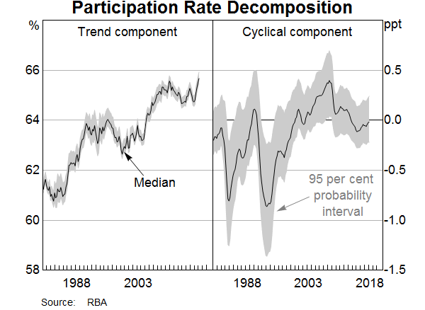
The results in Graph 3 confirm that the upward trend in the participation rate over recent decades has largely reflected structural factors. But, at times, the cyclical deviation from the trend component has been large. For example, during the recessions of the early 1980s and 1990s, the participation rate was around 0.75 percentage points below its long-run trend. The results suggest that the participation rate rose above its long run trend during the mid 2000s as rising commodity prices and the rapid expansion of the resources sector brought more people into the labour market. More recently, the participation rate is estimated to have been slightly below its long-run trend in recent years, which suggests there has been spare capacity in the labour market. The estimates suggest that the pick-up in the participation rate in the past year or so reflects both structural and cyclical factors, although it should be noted that estimates of the trend and cyclical components at the end of the sample are prone to revision as new data become available.
Whose Labour Force Participation Is Most Cyclically Sensitive?
The previous section described the cyclical behaviour of labour force participation across the economy as a whole. We now look at whether certain segments of the population differ in their ability and willingness to enter or leave the labour force in response to changing economic conditions.
As in the previous section, we need a way to separate the cyclical, demand-driven components of labour force participation from the longer-run, structural supply-driven components. Without a way to identify the cyclical components, our estimates of the response of the participation rate to changes in economic conditions would be too large because they would also include the effect of the supply-driven components. Our approach makes use of cross-state variation in labour market conditions by industry. This approach relies on three assumptions. The first is that demand conditions for individual industries are likely to be similar across states. For example, a rise in commodity prices that encourages mining firms to expand production and hire more workers in Queensland is also likely to increase mining production and employment in Western Australia. The second is that changes in the supply of labour in one state do not materially affect employment in other states. For example, if more people in New South Wales choose to enter the labour force, this will not have a large effect on employment in Victoria, even if it raises employment in New South Wales. The third is that participation rate responses are the same across states. If these assumptions are correct, we can use changes in industry-level employment in other states as proxies, or instruments, for changes in labour demand in the relevant state. Details of our empirical approach are in Appendix B.
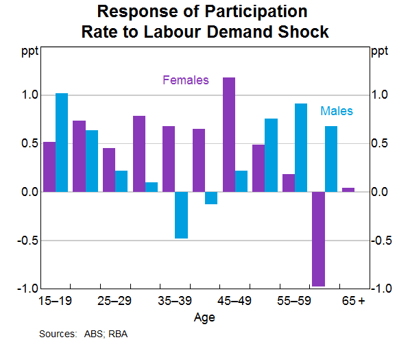
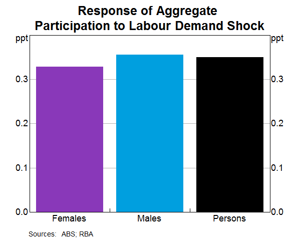
Graph 4 shows our estimates of cyclical sensitivity of participation rates for each five-year age group and sex.[7] Each bar shows the response of a group to a one per cent increase in the demand for labour, based on this identification strategy. A larger positive bar indicates that a group's labour supply increases by more than others following an improvement in economic conditions. We find that younger workers of both sexes, 25–54-year-old females and older males are most responsive to changes in labour demand. In contrast, males aged 25–54 years are less likely to alter their labour force participation in response to changing economic conditions.[8] The large negative estimate for 60–64-year-old women is surprising, but is imprecisely estimated and the estimate is not significant at any conventional level. As such, we do not read too much into this result. Grouping all of the age groups together, we find that a 1 per cent increase in labour demand leads to slightly more than a 0.3 percentage point increase in the aggregate participation rate (Graph 5), which is consistent with our findings in the previous section. In aggregate, the responsiveness of males and females are nearly identical.
We also explore whether the cyclical sensitivity of participation decisions has changed over time. There are a number of reasons why such a change might have occurred. For example, firms increasingly adjust to changes in demand by altering the hours worked of individual workers, rather than the number of workers they employ, perhaps due to changes in the flexibility of the Australian labour market (Bishop, Gustafsson and Plumb 2016). If fewer workers become unemployed during recessions, we might also expect fewer workers to leave the labour force, potentially reducing the cyclical responsiveness of workers' participation rates. The large increase in female participation over recent decades and the increasing prevalence of part-time work mean that the characteristics of those who are employed, and the cyclical sensitivity of their labour force participation, may differ from three decades ago. Other factors, such as the level of debt held by a household, or declines in net wealth near retirement, also influence labour force participation decisions (Belkar, Cockerell and Edwards 2007). Long-term trends in these variables, or recent large events such as the global financial crisis, may also have changed the sensitivity of labour force participation to economic conditions. For instance, workers' participation decisions may have become less sensitive to cyclical conditions if higher household debt means they must work in order to service their debt.
To test for evidence of changes in the responsiveness of participation rates to economic conditions, we repeat the exercise in Graph 4, splitting our sample into two periods, pre- and post-June quarter 1998. This date broadly coincides with a decline in the volatility of GDP growth in Australia and follows a period of labour market reforms in the 1980s and 1990s (Bishop et al 2016).
We find that the differences between the two samples mostly point to increased sensitivity to labour market conditions in the recent sample for all groups, other than for older workers.[9] However, the differences are for the most part small, and not statistically significant. The increases are somewhat larger for females, although not statistically significantly different from the increase for males. We view this exercise as providing only tentative evidence that labour force participation has become more cyclically sensitive over time.[10]
Macroeconomic Consequences of Cyclical Changes in the Participation Rate
To explore how shifts in labour force participation affect the economy's adjustment to changes in the level of economic activity, we use MARTIN, the RBA's macroeconometric model.[11] Using MARTIN allows us to trace through the implications of an increase in aggregate demand first to economic activity and the labour market and then from these variables to prices and wages. The model also accounts for interactions and feedbacks between all of these variables.
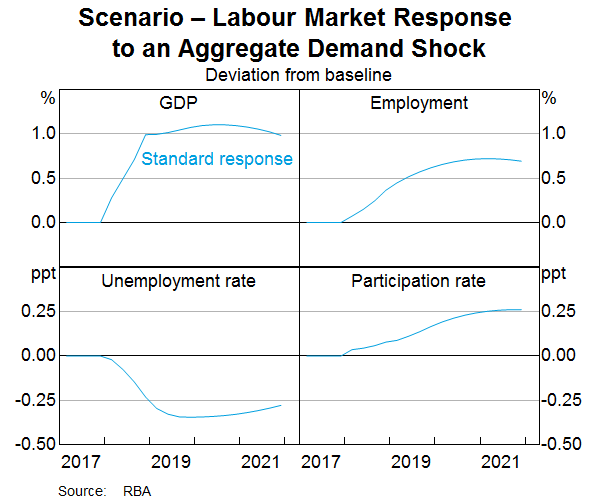
We compare two scenarios. In the first scenario, an unanticipated increase in aggregate demand boosts the level of economic activity by one per cent for three years, and the labour market is assumed to respond in its usual way.[12] We hold the cash rate and the real exchange rate fixed in this scenario, allowing us to examine the consequences of a change in aggregate demand independently of the effects of monetary policy.
An increase in aggregate demand encourages firms to hire more workers (Graph 6). Labour market outcomes are typically thought to lag the business cycle, reflecting the time it takes for firms to hire workers and adjust their work practices to accommodate a larger workforce. Consistent with this, employment responds more slowly than output to the pick-up in demand, increasing by 0.7 per cent after three years. As suggested by Graph 2, the increase in employment is met in part by a fall in the unemployment rate and in part by a cyclical rise in the participation rate. The relative responses of these two variables are broadly in line with the relationships described above.
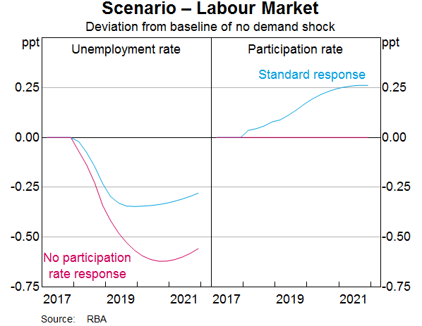
For the second scenario, we impose the same increase in aggregate demand, but ensure that the participation rate does not respond to the increase in demand. Once again, we hold the cash rate and the real exchange rate fixed in this scenario. Economic activity and labour demand both pick up by roughly as much as in the first scenario. But now all of the adjustment to a higher level of employment comes through a fall in the unemployment rate (Graph 7).
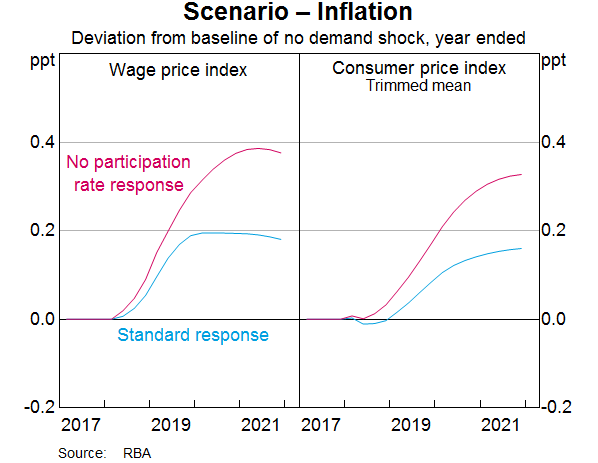
The effects of the two scenarios on real variables, like output and consumption, are similar. But they have very different implications for nominal variables, like inflation. In both scenarios, the increase in aggregate demand causes a pick-up in nominal wages growth and inflation (Graph 8). But without the participation rate response, the inflationary effects are much larger. For example, in the first scenario the increase in aggregate demand raises nominal wages growth by around 0.2 percentage points after two years. In the second scenario, where the participation rate is constant, the increase in nominal wages growth is closer to 0.4 percentage points. However, the difference in real wages growth, which is ultimately what determines the increase in living standards, is relatively small between the two scenarios, because inflation also increases by more when the participation rate does not respond.
The larger response of prices and wages when the participation rate does not respond is consistent with people who are actively seeking work (and hence counted in the unemployment rate) exerting a larger dampening influence on wages growth than they would if they were outside the labour force. Because increased participation provides a larger boost to effective labour supply, the two scenarios have different effects on wages and inflation even though employment growth is the same.[13]
The two scenarios illustrate the important role that changes in labour force participation play in helping to mitigate the economic effects of changes in aggregate demand. Without adjustments in the participation rate, economic expansions would be more inflationary. In response, the cash rate would need to be higher than otherwise, potentially limiting the size and duration of economic expansions. Although we have focussed on scenarios in which aggregate demand increases, similar mechanisms would also be at play if aggregate demand declined. In this environment, without adjustment through changes in the participation rate, the resulting downturn would be more disinflationary and lead to larger increases in involuntary unemployment. In this sense, the cyclical component of the participation rate acts as a stabiliser, limiting the inflationary effects of changes in aggregate demand.
Conclusion
Over the long run, changes in labour force participation are largely driven by structural factors. But in the short run, the participation rate also has a large cyclical component. When economic conditions strengthen, more people, especially young people, 25–54-year-old females and older males, enter (or delay leaving) the labour force. When economic conditions weaken, the labour force participation of these groups declines. Changes in the participation rate are an important part of the economy's adjustment mechanism to changes in the level of aggregate demand.
Appendix A: Estimating the Statistical Model
The model consists of equations linking the level of GDP per capita, the unemployment rate and the participation rate to their trends and the business cycle.
GDP per capita:
Unemployment rate:
Participation rate:
where is the level of GDP per capita, is the unemployment rate and is the labour force participation rate. The model also includes equations for the unobserved state variables: potential output, , the trend level of unemployment, , the trend participation rate, , and the business cycle, :
where and are shock processes with the variance-covariance matrix :
We estimate our model over the period March quarter 1966 to March quarter 2018. We allow for a break in the parameters of in 1984Q1 to account for the reduction in macroeconomic volatility since the middle of the 1980s.
We estimate the model using Bayesian methods. This allows us to combine prior information about the values of the estimated parameters from economic theory and other studies with information from the data. Intuitively, the estimation procedure searches for the combination of parameter values that best explains the observed behaviour of GDP per capita, the unemployment rate and the participation rate but penalises parameter estimates that are far from our expectations. The size of the penalty depends on the strength of our ‘priors’. If we have strong reasons to believe that a parameter falls in a particular range, the penalty for deviating from that range will be large. For other parameters, where our beliefs are not as strong, the penalty will be small. For example, economic theory and empirical evidence strongly suggests than an improvement in economic conditions will lower the unemployment rate. Therefore, our priors favour parameter estimates that imply a negative correlation between the level of the unemployment rate (relative to the NAIRU) and the business cycle.
For a given set of parameter estimates, we use a statistical technique known as the Kalman filter to generate estimates of the unobserved variables. At each observation in the sample, given an estimate of these variables and Equations (A1) – (A7), the model will produce a prediction for GDP per capita, the unemployment rate and inflation. Any differences between the predictions and the actual data will cause some revision in the estimate of the trends and the business cycle for that quarter. Using these revised estimates, the process is then repeated for the next quarter. Once we reach the end of the sample, we use the Kalman smoother to construct estimates of the trends and cycle based on the full history of the data. We construct the cyclical component of the participation rate as the actual value of the participation rate minus the estimate of its trend component. Table A1 describes the data sources and Table A2 describes the prior distributions and estimation results.
| Variable | Description | Source |
|---|---|---|
| Real GDP per working-age person | ABS cat. 5206.0 | |
| Trend GDP per working-age person | ||
| Business cycle | ||
| Unemployment rate | ABS cat. 6202.0 | |
| Trend unemployment rate | ||
| Labour force participation rate | ABS cat. 6202.0 | |
| Trend labour force participation rate | ||
|
Source: RBA |
||
| Parameter | Posterior | Distribution | Prior | ||
|---|---|---|---|---|---|
| Mode | Mean | Mean | Standard deviation | ||
| Structural Parameters | |||||
| −0.86 | −0.97 | Normal | −0.5 | 1.0 | |
| −0.37 | −0.40 | Normal | −0.5 | 1.0 | |
| −0.26 | −0.25 | Normal | 0.5 | 1.0 | |
| 0.59 | 0.73 | Normal | 0.5 | 1.0 | |
| 0.39 | 0.39 | Uniform | |||
| 0.99 | 0.98 | Beta | 0.5 | 0.3 | |
| −0.75 | −0.74 | Normal | −0.5 | 1.0 | |
| Shock Processes | |||||
| 1.27 | 1.30 | Gamma | 1.0 | 0.8 | |
| 0.28 | 0.28 | Gamma | 1.0 | 0.8 | |
| 0.40 | 0.40 | Gamma | 1.0 | 0.8 | |
| 0.16 | 0.19 | Gamma | 1.0 | 0.8 | |
| 0.85 | 0.73 | Beta | 0.5 | 0.3 | |
| 0.58 | 0.58 | Gamma | 1.0 | 0.8 | |
| 0.16 | 0.16 | Gamma | 1.0 | 0.8 | |
| 0.31 | 0.30 | Gamma | 1.0 | 0.8 | |
| 0.10 | 0.11 | Gamma | 1.0 | 0.8 | |
| 0.42 | 0.36 | Beta | 0.5 | 0.3 | |
| Memo Item | |||||
| 0.39 | 0.47 | ||||
|
Source: RBA |
|||||
Appendix B: Estimating Group-level Participation Rate Cyclical Sensitivity
To estimate how participation rates respond to labour demand, we estimate the following state-level panel regression for each five-year age and sex group , and aggregate participation rates by sex:
- is the quarterly percentage point change in the participation rate of age and sex group in state in quarter
- is quarterly employment growth in state in quarter
- are state fixed effects
- is the coefficient of interest for each five-year age and sex group. It is the response of the group's participation rate to a 1 per cent labour demand shock.
Because employment growth and the participation rate are jointly determined by labour demand and labour supply, Equation (1) faces an endogeneity problem and so would provide a biased estimate of . To address this issue, we need an instrument for employment growth that is correlated with labour demand shocks, but uncorrelated with labour supply shocks. We use the industry shift-share instrument from Bartik (1991) and Blanchard and Katz (1992):[14]
- is the industry-share instrument in state in quarter
- is the industry division share of employment of industry in state in the previous quarter
- is aggregate employment growth in industry division for Australia excluding state
The instrument predicts labour demand in a state from the lagged industry composition of the state and industry-level employment growth in all other states. This approach assumes that, at an industry level, demand conditions are likely to be similar across states. For example, a rise in commodity prices that leads to an increase in mining employment in Queensland is likely to have the same effect on mining employment in Western Australia. Because WA has a (relatively) large share of its employment in mining, the instrument predicts that overall employment growth in WA will be strong. The key identification assumption is that labour supply shocks in state do not affect industry employment growth in any of the other states.
Participation rate and employment data come from the monthly detailed labour force statistics; we use quarterly averages and seasonally adjust the data because the five-year age group data are published in original terms. Industry employment data is from the detailed quarterly labour force statistics. Our sample runs from March quarter 1985 to March quarter 2018.
We then estimate the response to labour demand for each age and sex group using two-stage least squares using as an instrument for state-level employment growth, . Table B1 shows the estimated coefficient values and standard errors.
| Females | Males | Females | Males | |||
|---|---|---|---|---|---|---|
| 15–19 | 0.52*** | 1.02*** | 45–49 | 1.18*** | 0.22** | |
| (0.16) | (0.23) | (0.36) | (0.11) | |||
| 20–24 | 0.74*** | 0.63*** | 50–54 | 0.49** | 0.76** | |
| (0.25) | (0.20) | (0.23) | (0.30) | |||
| 25–29 | 0.46** | 0.22* | 55–59 | 0.18 | 0.91*** | |
| (0.20) | (0.12) | (0.38) | (0.23) | |||
| 30–34 | 0.78*** | 0.10 | 60–64 | −0.97 | 0.68 | |
| (0.17) | (0.13) | (0.66) | (0.57) | |||
| 35–39 | 0.68*** | −0.48* | 65+ | 0.04 | 0.00 | |
| (0.24) | (0.27) | (0.06) | (0.12) | |||
| 40–44 | 0.65*** | −0.12 | ||||
| (0.17) | (0.19) | |||||
|
***, ** and * denote statistical significance at the 1 per cent, 5 per cent and 10 per cent levels. Sources: RBA |
||||||
Footnotes
The authors are from Economic Analysis Department [*]
Connolly, Davis and Spence (2011) and RBA (2013) discuss long-run trends in the participation rate in more detail. [1]
We plot the change in the employment-to-population ratio rather than employment growth to abstract from the part of employment growth that comes mechanically from increases in the size of the population. Plotting these relationships in quarterly changes produces a similar pattern. [2]
If this were not the case, the increase in the participation rate over the past 40 years would have been associated with a rise in the non-accelerating inflation rate of unemployment (NAIRU). The evidence presented in Cusbert (2017), however, suggests that the NAIRU has fallen over this time. [3]
The relationship between changes in the employment-to-population ratio and changes in the unemployment rate is almost one-for-one. However, because the denominator of the employment-to-population ratio (the working-age population) is larger than the denominator of the unemployment rate (the labour force), a 1 percentage point fall in the unemployment rate is too small to fully account for a 1 percentage point increase in the employment-to-population ratio. [4]
The model's estimates of the NAIRU are broadly similar to those described in Cusbert (2017). The estimates of potential output growth imply a business that accords with standard accounts of Australia's economic performance over recent decades, with large recessions in the early 1980s and early 1990s. [5]
There are two main sources of uncertainty around the estimates. The first is uncertainty about the relationship between the participation rate and the economic cycle, which may be stronger or weaker than the central estimates imply. The second is uncertainty about the economic cycle, which may be closer to or further away from its trend than the central estimates imply. [6]
A table of coefficient estimates and standard errors can be found in Appendix B. [7]
These results are consistent with the extensive overseas literature on the cyclical sensitivity of labour force participation by age and sex, including Rones (1983), Leppel and Heller Clain (1995) and (Benati 2001). Earlier Australian studies by Debelle and Vickery (1998) and O'Brien (2011) reached similar conclusions. [8]
Using an earlier sample, Lenten (2000) also finds that participation rates have become more cyclical over time. [9]
Other cyclical labour market relationships, for example, the relationship between output growth and the unemployment rate also appear to have been stable over time (see Lancaster and Tulip (2015)). [10]
See Cusbert and Kendall (2018) for a description of MARTIN. [11]
We simulate the increase in aggregate demand through an unanticipated increase in government expenditure. The implications for the labour market, wages and inflation are similar if the increase in aggregate demand comes via an increase in household consumption. [12]
This is a key assumption in MARTIN. It is supported by empirical evidence that the movements in the unemployment rate better describe wages growth than changes in employment. [13]
We exclude the ACT, as it is missing industry employment data in some periods for some industries. [14]
References
Bartik T (1991), Who Benefits from State and Local Economic Development Policies?, W.E. Upjohn Institute, pp 1–16.
Belkar R, L Cockerell and R Edwards (2007), ‘Labour Force Participation and Household Debt’, RBA Research Discussion Paper No 2007-05.
Benati L (2001), ‘Some Empirical Evidence on the “Discouraged Worker” Effect’, Economics Letters, 70, pp 387–395.
Bishop J, L Gustafsson and M Plumb (2016), ‘Jobs or Hours? Cyclical Labour Market Adjustment in Australia’, RBA Research Discussion Paper No 2016—06.
Blanchard O and L Katz (1992), ‘Regional Evolutions’, Brookings Papers on Economic Activity, 1, pp 1–75.
Connolly E, K Davis and G Spence (2011), ‘Trends in Labour Supply’, RBA Bulletin, June, pp 1–8.
Cusbert T (2017), ‘Estimating the NAIRU and the Unemployment Gap’, RBA Bulletin, June, pp 13–22.
Cusbert T and E Kendall (2018), ‘Meet MARTIN, the RBA's New Macroeconomic Model’, RBA Bulletin, March, viewed 5 September 2018.
Debelle G and J Vickery (1998), ‘The Macroeconomics of Australian Unemployment’, in G Debelle and J Borland (eds), Unemployment and the Australian Labour Market, Reserve Bank of Australia Conference, pp 235–265.
Lancaster D and P Tulip (2015), ‘Okun's Law and Potential Output’, RBA Research Discussion Paper No 2015—14.
Lenten L (2000), ‘The Profile of Labour Discouragement in Australia’, Australian Journal of Labour Economics, 4(1), pp 3–17.
Leppel K and S Heller Clain (1995), ‘The Effect of Increases in the Level of Unemployment on Older Workers’, Applied Economics, 27, pp 901–906.
O'Brien M (2011), ‘Discouraged Older Male Workers and the Discouraged Worker Effect’, Australian Journal of Labour Economics, 14(3), pp 217–235.
RBA (2013), ‘Box C: The Labour Force Participation Rate’, RBA Statement on Monetary Policy, February, pp 40–42.
Rones P (1983), ‘The Labor Market Problems of Older Workers’, Monthly Labor Review, 1983(May), pp 2–12.
van der Merwe M (2016), ‘Factors Affecting an Individual's Future Labour Market Status’, RBA Bulletin, December, pp 11–22.


