RBA Annual Conference – 2005 International Business Cycle Co-movements through Time Dan Andrews and Marion Kohler[1]
1. Introduction
The increasing integration of the world economy in recent decades, through the liberalisation of trade and capital flows, has raised the possibility of a more rapid transmission of business cycle fluctuations across countries, especially those originating in large economies such as the United States. Indeed, over the past 40 years, the Australian and US business cycles have become highly correlated, a point well documented in the literature and exploited in a number of macroeconomic models for Australia.[2] Table 1 shows output correlations between Australia and a number of industrialised economies over the past 40 years.[3] It illustrates that the business cycle relationship between Australia and the US is not the only one which has changed over time.
| Australia with: | Correlation of real GDP (year-ended growth rates) |
Correlation of GDP cycles (band-pass filtered) |
|||||
|---|---|---|---|---|---|---|---|
| 1961:Q1–2004:Q4(a) | 1961:Q1–1982:Q4(a) | 1983:Q1–2004:Q4 | 1963:Q1–2001:Q4(b) | 1963:Q1–1982:Q4(b) | 1983:Q1–2001:Q4 | ||
| (a) Sample for Canada starts in 1962:Q1, for the euro
area in 1971:Q1 and for New Zealand in 1978:Q1. (b) Sample for Canada starts in 1964:Q1, for the euro area in 1973:Q1 and for New Zealand in 1980:Q1. |
|||||||
| Canada | 0.51 | 0.38 | 0.66 | 0.58 | 0.25 | 0.83 | |
| Euro area | 0.23 | 0.40 | 0.16 | 0.32 | 0.46 | 0.21 | |
| Japan | 0.28 | 0.41 | 0.00 | 0.30 | 0.49 | 0.07 | |
| New Zealand | 0.29 | – | 0.21 | 0.38 | – | 0.32 | |
| UK | 0.27 | 0.19 | 0.50 | 0.28 | 0.06 | 0.60 | |
| US | 0.34 | 0.23 | 0.59 | 0.31 | 0.02 | 0.82 | |
While previous studies have sought to explain business cycle correlations in a cross-country context, less is known about the factors which have caused these relationships to change dramatically through time. This paper aims to analyse the extent to which cross-sectional explanations of business cycle co-movements can also explain changes in co-movements over time.
We find that the changes in cycle co-movement can – at least partly – be explained by factors similar to those highlighted in cross-sectional studies, such as trade and industrial structure. We also find a role for a measure of market flexibility and for monetary and fiscal policy for some economy pairs. However, the exact model and the sign of the effect of different factors on cycle co-movement varies across economy pairs.
In Section 2 we document the changes in the co-movements of Australia's business cycle with those of the economies in Table 1 in more detail. In Section 3 we analyse graphically how the explanatory factors proposed in the cross-sectional literature have evolved through time for our economy pairs and test the influence of these factors over time more formally. In Section 3.3, we briefly consider financial integration as an alternative explanation, before concluding in Section 4.
2. Business Cycle Co-movements through Time
In this section we document the changes in Australia's international business cycle co-movements in more detail. Figure 1 shows the growth cycles of real GDP for Australia and the US over the past 45 years.
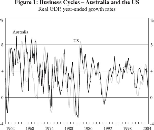
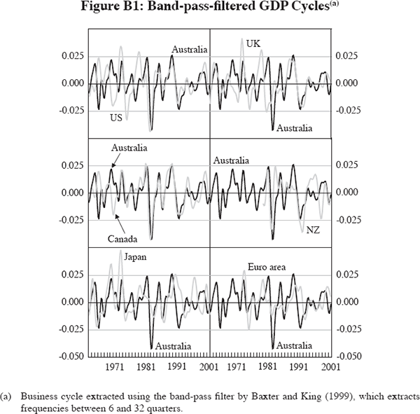
A first glance confirms that the GDP cycle of Australia was less synchronised with that of the US in the earlier part of the sample, while it became highly synchronised after 1980. One way to measure this synchronisation and to capture co-movement over the entire cycle is to calculate correlation coefficients over some period, for instance 16 years, which captures on average roughly two cycles.[4] We calculate the bilateral correlation of these cycles using correlation coefficients over 16-year moving windows over the sample period. We use a slightly different definition of the business cycle based on the cyclical component of quarterly real GDP, isolated using the band-pass filter proposed by Baxter and King (1999).[5] The corresponding charts of the cycles for all economy pairs can be found in Appendix B.
Figure 2 shows the change in business cycle co-movement between Australia and the US, and between Australia and the United Kingdom. The dates on the chart show the end-dates of the moving window, so that the first data point covers the correlation over the time period 1963:Q1 to 1978:Q4 and the last data point covers the time period 1986:Q1 to 2001:Q4.
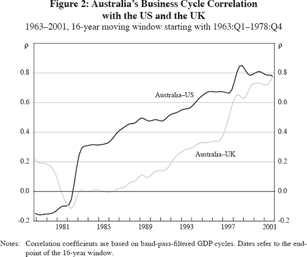
Quite remarkably, the correlation with the US has increased from around zero (that is, uncorrelated) before 1980 to around 0.8 towards the end of the sample period. While the increase has mostly been gradual, a step increase can be observed in the mid 1980s, partly driven by the coincident recessions in the early 1980s in both countries. The business cycles of the two countries have been in close synchronisation for the following 20 years (though the US experienced a recession in 2001 while Australia did not). This suggests that structural changes might have occurred that increased the economic links between the two economies.
Figure 2 also documents the change in the co-movement of the Australian and the UK business cycles. Despite the close historical ties of the two economies, the cycles were uncorrelated throughout most of the 1960s, 1970s and 1980s. However, already in the early 1980s a gradual increase in the correlation of cycles is apparent, reaching 0.8 at the end of the sample. One reason for this increase could be the transmission of shocks via a third country, such as the US, rather than ‘direct’ transmission between Australia and the UK. This may partly reflect the fact that the correlation between the US and the UK cycles has always been at a high level. However, it has been decreasing between the 1970s and the mid 1990s from 0.75 to 0.5, while the Australia–UK correlation jumps up later in the sample period, suggesting that other factors may be driving the increase in the correlation with Australia.
Figure 3 depicts the correlation of the Australian cycle with that of Canada and New Zealand (plus, for comparison, that with the US). Canada is an interesting case for several reasons. First, its economy is known to have close ties with the US economy, with a correlation at or above 0.8 for the past 40 years, one of the highest among OECD countries. Second, like Australia, Canada is a small open economy with a large share of commodity exports. Interestingly, Australia's correlation with the Canadian cycle is even higher than it is with the US. Similar to the US cycle correlation, it has increased over the sample period, but it did so earlier and remained flat at a high level for the past two decades.
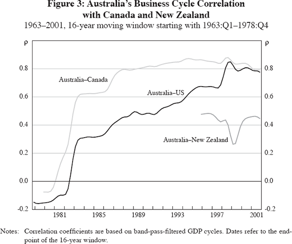
One might suspect that the high correlation of the Australian and Canadian cycles is due to their common exposure to world commodity cycles. However, the correlation with New Zealand, another small open economy with significant commodity exports and one that trades more intensively with Australia, is much lower. Unfortunately, data limitations do not allow us to investigate whether this correlation changed at the same time that the correlation with Canada changed. Surprisingly, despite the shorter sample period and the overlapping windows used for the rolling correlations, the correlation drops significantly around the Asian financial crisis in 1997–98, indicating how disruptive this event was for New Zealand relative to Australia.
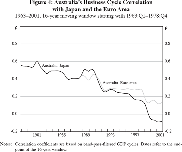
Finally, Figure 4 shows the correlation of Australia's cycle with that of two major industrialised trading partners, Japan and the euro area. Both are relatively low in the second half of the sample, consistent with the existence of an Anglo-Saxon effect in business cycle correlations identified by Otto et al (2001). However, the correlation with Australia used to be higher in the earlier part of the sample, especially in the case of Japan. This fall in correlations could be due, in part, to the idiosyncratic shocks experienced by Japan and the euro area over the 1990s.[6] However, we will analyse in the next section whether other, structural, factors may also have been at work.
3. Explaining Business Cycle Co-movements
3.1 Evidence from cross-sectional studies
As the previous section demonstrates, Australia's business cycle has become more correlated with some countries, and less so with others. Business cycles, and their synchronisation across countries, are determined by the interaction of common shocks, country-specific or idiosyncratic shocks, and the transmission of these shocks within countries. By themselves, common shocks will tend to lead to synchronisation of business cycles across countries. Even in the presence of significant common shocks, however, business cycles may diverge due to differences in the (domestic) transmission of shocks. Differences in transmission are in turn likely to reflect structural differences, including the structure of industry, labour and product markets, and of the financial system. Country-specific shocks, which are essentially the result of border effects, such as differences in the stance of fiscal and monetary policies, will tend to reduce synchronisation of business cycles. Finally, in the open-economy context, business cycles can be correlated if country-specific shocks are transmitted across borders, thus acting like a common shock. One key vehicle for this international transmission is trade. Consequently, the cross-sectional studies that aim at explaining business cycle co-movement have focused on these structural factors: trade; industrial structure; adjustment mechanisms to shocks; and monetary or fiscal policy reactions. More recently, a number of studies have sought to exploit financial market integration to explain business cycle co-movement, a point we will return to in Section 3.3. We will now discuss each of the structural factors in turn.
3.1.1 Trade
Trade has become an important theme in the literature, especially since Frankel and Rose (1998) found that countries with closer trade links tend to have more closely correlated business cycles. Theoretically, however, the effect of trade on synchronicity is ambiguous. Krugman (1993) argues that a pair of countries that trade more may specialise more in order to reap the gains from trade. This would lead to even greater differences between each country's industrial structure, and in the presence of sector-specific shocks (even if these are common across countries) it can lead to more idiosyncratic business cycles. The importance of this effect depends upon the degree of specialisation induced by trade integration, which tends to rise with the ratio of inter-industry to intra-industry trade. Furthermore, the net effect on business cycles depends upon the relative importance of aggregate and sector-specific shocks. If the relative variance of aggregate shocks is greater than that of sector-specific shocks, closer trade integration could be expected to lead to more synchronised business cycles (Frankel and Rose 1998).
Much of the recent literature can be defined in terms of its efforts to establish a more robust relationship between trade and synchronicity (Clark and van Wincoop 2001, Imbs 2000, Otto et al 2001). After controlling for other factors, especially industrial structure, these studies generally find that the effect of trade is small and positive (Imbs 2000), or in some cases, insignificantly different from zero (Otto et al 2001). In recent work, Baxter and Kouparitsas (2005) argue that only bilateral trade has a robust (and positive) coefficient in explaining business cycle co-movements across countries.[7]
Following much of the literature we use a number of different measures for bilateral trade exposure.[8] The first measure, following Frankel and Rose (1998), is the bilateral trade share, that is, total bilateral trade relative to total trade of the two economies i and j:

The second measure, used by Frankel and Rose (1998) and Clark and van Wincoop (2001), is bilateral openness, which takes into account the possibility that bilateral trade exposure may matter more for GDP fluctuations in relatively open economies, which tend to be small, than in relatively closed economies, which tend to be large. Bilateral openness is defined as the ratio of bilateral trade to the sum of nominal GDP in the two economies i and j:

The trade measures so far are symmetric for the two economies. However, we could imagine that there is a one-way interdependence in the case of a small economy, such as Australia's, trading intensively with a very large economy, such as that of the US. Then the trade share from the perspective of Australia might matter more than some average of both trade shares. Measures that capture such an asymmetry have been used by Kose, Prasad and Terrones (2003) and Otto et al (2001). Therefore, we also consider a trade share measure, which is defined as bilateral trade over total Australian trade.[9]

A number of studies address the potential endogeneity of trade and cyclical correlation by including elements of the gravity model to instrument for trade. Unfortunately, this is difficult to do in our study, since variables such as the distance of two economies are time-invariant, and therefore unsuitable for our time-series model.
3.1.2 Industrial structure
Industry-specific shocks account for a considerable share of global shocks (see, for example, Clark and Shin 2000, Funke, Hall and Ruhwedel 1999, and Kwark 1999). Economies with a similar industrial structure will tend to transmit and receive these common shocks in a similar fashion, and consequently experience co-movements of their business cycles. Not surprisingly, a number of authors have included measures of industrial structure in their cross-sectional studies. Clark and van Wincoop (2001), Imbs (1999) and Kalemli-Ozcan, Sørensen and Yosha (2001) all argue that more similar production structures lead to higher correlation, and Imbs (1999) finds that the effect of industry similarity on cycle co-movement is larger than that of trade.
To measure dissimilarity in industry specialisation, we adopt Krugman's (1991)
index, which aggregates the absolute difference of sectoral output shares,
 , across all sectors. Sectoral output shares are
defined as the value-added share of sector k,
  , in total value added,
  . The index of dissimilarity in industry specialisation
is:

This takes values between zero and two, with higher values indicating sectoral dissimilarity. We choose a broad sectoral breakdown, which covers the 10 one-digit industries in the International Standard Industrial Classification (ISIC).[10]
3.1.3 Market flexibility
Differences in market structure – particularly with regard to the flexibility of markets – might be an important factor in explaining the degree of cyclical co-movement, since it can measure the adjustment of an economy to a shock. Countries with similar market structures could be expected to react similarly to a common shock. Of course, the effect of relative market flexibility on business cycle co-movement is not unambiguous, but it will also depend on the level of market flexibility. More flexible economies could be expected to adjust more rapidly to large idiosyncratic shocks, thereby dampening their impact on the business cycle. This would tend to lead to greater co-movement of business cycles. Therefore, the overall effect of changes in market flexibility will depend not only on relative market flexibility, but also on the prevalence of different types of shocks.
The aspect of adjustment to shocks within economies has been relatively neglected in the cross-sectional literature. Otto et al (2001) use indices of market structure that capture accounting standards and concentration of firm ownership. They find evidence of an ‘Anglo-Saxon effect’ which they explain by factors such as common legal institutions, accounting standards and technology take-up. However, these are likely to change little over time, and are therefore probably more suitable to explain cross-sectional differences, than those over time. An economy's ability to adjust to idiosyncratic shocks has received more prominence in the context of cyclical co-movements within the European Monetary Union, starting with the influential work by Bayoumi and Eichengreen (1993). However, few studies have explicitly modelled structural factors that explain adjustment, possibly because of a lack of suitable data.
Measuring market flexibility, especially over time, is an even more difficult task. Following Blanchard and Wolfers (2000), we have chosen a measure of net union density to proxy labour market flexibility. While this cannot capture all aspects of labour market flexibility, or market flexibility, we will show below that its time profile lines up reasonably well with the index of product market flexibility developed by Nicoletti et al (2001) and used by Kent, Smith and Holloway (this volume). In order to capture the difference in labour market flexibility (LMF) between two economies, we use two measures. The ratio of net union density (NUD) is used for the graphical analysis, where ‘similarity’ implies a value of one:[11]

Following the definition of dissimilarity for other variables in our model, we use the absolute difference in net union density in the regressions, where ‘similarity’ implies a value of zero:

3.1.4 Monetary and fiscal policy
In the context of monetary unions, much attention has been paid to the effect of the co-ordination of monetary and fiscal policies on business cycle synchronisation. To the extent that monetary and fiscal policy shocks in an individual economy are a source of business cycle movements, a common policy across countries would lead to higher business cycle co-movement. More similar policy reactions lead also to higher cycle synchronisation if economies are affected by a common, or rapidly transmitted, shock. On the other hand, an idiosyncratic response in policy can lead to more synchronisation by dampening country-specific shocks.
The empirical success of including policy differences to systematically explain differences in cycle co-movements across country-pairs has been mixed. Clark and van Wincoop (2001) cannot find a significant effect of policy on cycle synchronisation, but argue that this might be a result of policy being both a source of shocks and a stabiliser. On the other hand, Otto, Voss and Willard (2003) argue that similar monetary policy can be an important factor in business cycle synchronisation. Since changes in the similarity of fiscal or monetary policy may play a role in explaining changes in cycle synchronisation for a specific economy pair, we include such measures as possible controls in our considerations.
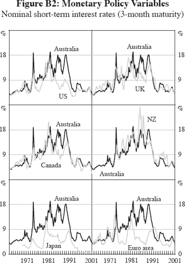
Similar to Clark and van Wincoop (2001) we measure monetary policy differences by taking the absolute difference of the nominal short interest rate (in our case, an interest rate with 3-month maturity):[12]

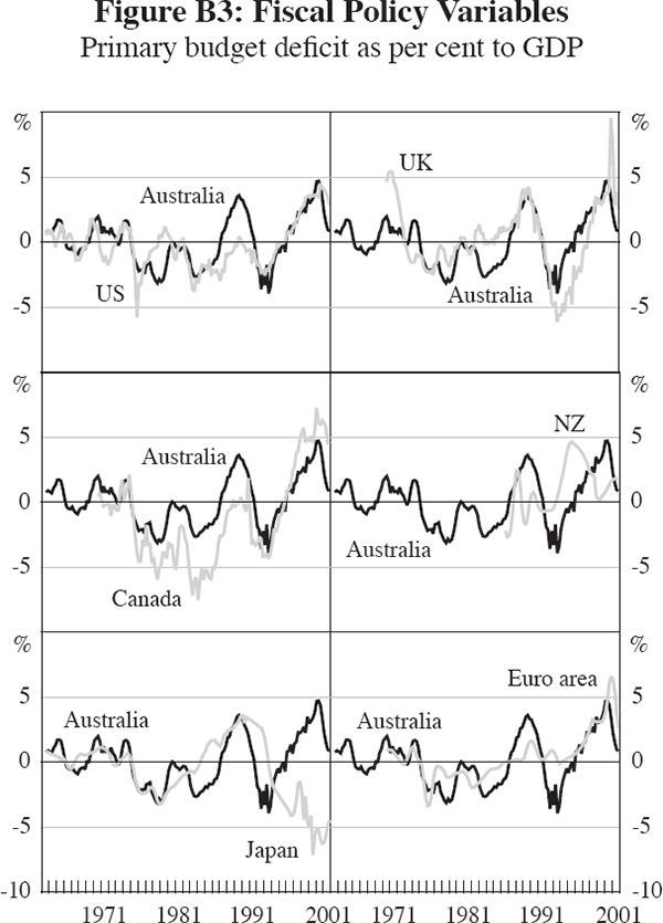
Fiscal policy similarity is measured by taking the absolute difference of the ratios of the primary budget balance to GDP:

3.2 Empirical evidence through time
In this section we analyse how the factors described in Section 3.1 have evolved over time for the economy pairs presented in Section 2. We will start with a graphical analysis, which allows us to gauge in which direction each of these factors may have affected business cycle synchronisation, if at all. We then proceed to a more formal test of whether these cross-sectional explanators can account for changes in cycle synchronisation over time.
3.2.1 Trends in factors through time
We use time-series data starting in 1963, or as far back as available, for our economies to construct the structural variables discussed in Section 3.1.[13] Details of the underlying data sources can be found in Appendix A.
The first economy pair under consideration is Australia and the US. Figure 5 shows the change in cycle synchronisation over time, and how the three factors, trade exposure, similarity of industrial structure and relative market flexibility have evolved through time.
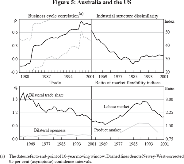
As noted above, the business cycle correlation between Australia and the US has increased strongly over the past 40 years. At the same time, however, the bilateral openness measure has increased only slightly and the bilateral trade share has fallen considerably. This implies, if anything, a negative relationship between cycle co-movement and trade, the opposite of what is suggested by cross-sectional studies. One explanation for this could be the dominance of Krugman-type effects, by which less bilateral trade can be a result of more similar industrial structures. In fact, this is supported by our industrial structure index which shows that the dissimilarity index has halved over the last 40 years, driven by the retail, manufacturing and government sectors.[14] Finally, labour market rigidities in Australia relative to the US have increased over the 1970s and 1980s, before falling to a level slightly above that in the 1960s. This hump-shaped profile hides falling labour market rigidities (as measured by net union density) in both countries: net union density fell in the US over the entire time period, while in Australia the trend decline in net union density began in the mid 1980s.
Of course, another possible explanation for the changes in cycle co-movement could be that the nature of the shocks to which both economies were exposed has changed. One example is the conduct of monetary and fiscal policy: both Australia and the US have changed the conduct of monetary policy considerably over the 1980s and the early 1990s. For Australia and the US, business cycles became more synchronised during the 1980s. However, this was also a period when monetary policy became – if anything – more idiosyncratic in the two economies with inflation falling earlier and remaining more stable much earlier in the US (detailed charts of the monetary policy and fiscal policy variables can be found in Appendix B). While monetary policy is an unlikely explanator for the changes in cycle co-movement between Australia and the US, we will see below that the conduct of policy may have played some role for other economy pairs.
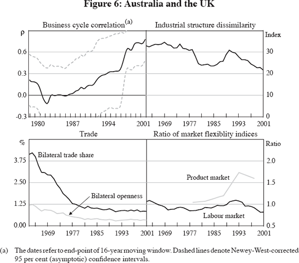
Australian business cycle co-movements with the UK have also increased over the last 40 years, although somewhat later than with the US. Both the bilateral trade share and bilateral openness have fallen sharply over the same period, again suggesting a negative relationship between trade and synchronicity (Figure 6). While the sectoral composition of the two economies has become more similar, the change is less dramatic than for the Australia–US pair, partly because the UK and Australia started at a more similar level. This suggests that a Krugman-type effect cannot be the entire explanation for the strong negative relationship between bilateral trade exposure and cycle co-movement. Also, market flexibility cannot shed more light on this, with the relative ratio of flexibility roughly flat around 1 over the period, which indicates that market flexibility has always been similar in the two economies through time.
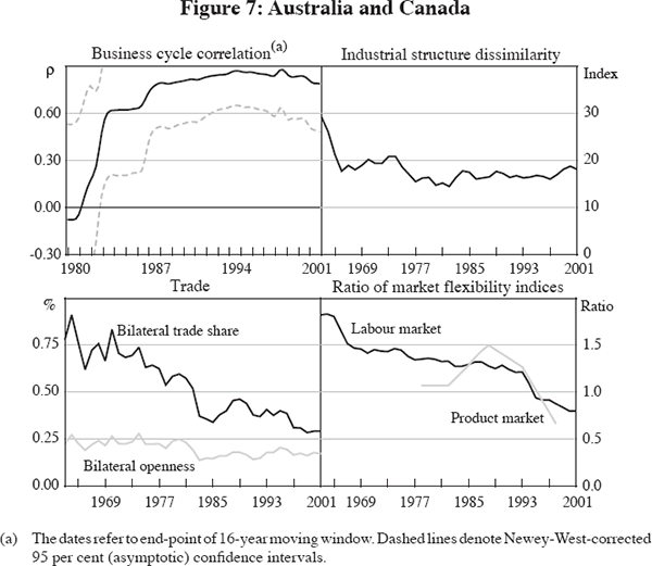
The increase in business cycle co-movements with Canada is one of the most striking, with much of the increase happening before the mid 1980s (Figure 7). Again, both measures of bilateral trade exposure have fallen over the period, although not to the extent seen in the previous two cases. Industrial structures became more similar early in our sample period and remained flat thereafter. In fact, Canada's industrial structure is the most similar to Australia in our selection of economies, partly providing an explanation for the high business cycle synchronicity. Relative labour market flexibility has also become more similar in the two economies, with Canada's net union density flat or slightly rising over the sample period, while that of Australia halved between the mid 1980s and 2002.
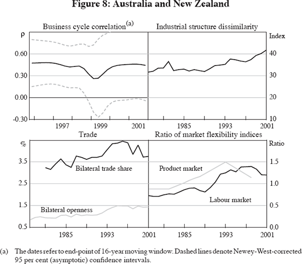
New Zealand's cyclical co-movement with Australia was broadly unchanged over the (much shorter) sample period. This contrasts with trend changes in our three explanatory factors (Figure 8). New Zealand is the only economy in our sample with a significant increase in bilateral trade exposure with Australia.[15] Similar to our previous cases, changes in trade exposure are accompanied by opposite changes in industrial similarity. In New Zealand's case, the sectoral composition has become more dissimilar to that of Australia, driven by the financial services, mining and manufacturing sectors. Labour market flexibility, as measured by net union density, is now very similar in the two economies, with the relative index increasing over time, driven by New Zealand's strong fall in net union density.
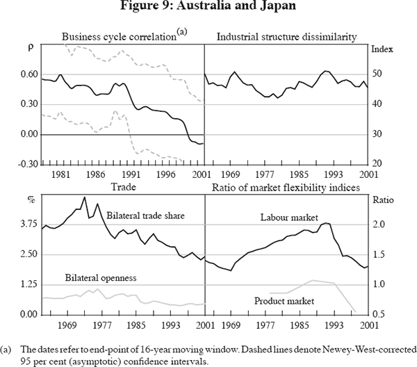
The cyclical correlation between Japan and Australia has fallen over the past 40 years (Figure 9). While part of this development, especially over the 1990s, is undoubtedly linked to strong adverse idiosyncratic shocks in Japan, it could also be partly explained by the underlying factors analysed here. More specifically, the fall in cycle correlation has been accompanied by a fall in bilateral trade exposure since the 1980s. Unlike the previous cases, the link between trade exposure and cycle correlation is positive in the case of Japan, as suggested by cross-sectional studies. Changes in industrial structure (dis-)similarity and relative labour market flexibility provide a less convincing explanation. Both have been roughly flat over the sample period, with relative labour market flexibility undergoing some swings.
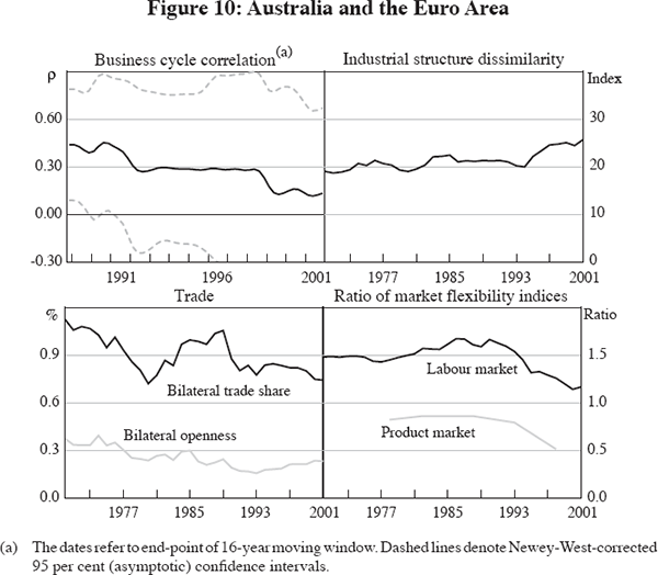
Similar to the case of Japan, the business cycle correlation between the euro area and Australia has fallen over the sample period (Figure 10). This is consistent with a fall in bilateral trade exposure, again suggesting a positive relationship between trade and synchronicity. Industrial structure has remained broadly unchanged, though the two economies have surprisingly similar structures when compared to Japan. Relative labour market flexibility changed significantly over the second half of the sample, with net union density broadly flat in the euro area while that of Australia halved over the same time. The level of net union density might be a somewhat misleading indicator of the level of market flexibility for the euro area. The product market indicator and other indicators of labour market flexibility by Nickell and Nunziata (2001) suggest that the economies of the euro area and Japan are more regulated than other economies in our sample. This implies a slower process of adjustment to shocks and might have contributed to the prolonged response to the idiosyncratic shocks these economies experienced in the 1990s (see Ebell and Haefke 2003).
Our analysis so far suggests that, while trade, industrial structure and market flexibility could explain changes in business cycle co-movements, the sign of these effects can differ widely across economy pairs. This is especially evident for trade exposure, which has a strongly negative correlation with cycle synchronicity for some countries, while it has a positive correlation for others. Interestingly, the first group, which includes the Anglo-Saxon countries, except for New Zealand, has had strongly increasing synchronicity with Australia despite falling bilateral trade exposure. For the UK and the US, we also find that industrial structure has become more similar, which may partly explain both the decreasing trade exposure and the increasing cycle co-movements. On the other hand, Canada's industrial structure has always been very similar, and therefore the strong increase in cycle co-movements is more difficult to explain.
The second group, Japan and the euro area, have experienced falling synchronisation of business cycles with Australia. This coincides with falling bilateral trade exposure, and a fall in relative labour market flexibility towards more similarity in the case of the euro area. Industrial structure similarity is an unlikely explanation for this group, as it has been roughly constant through time.
Ultimately, the relative importance of these factors for each economy pair needs to be established in an estimation which includes all factors jointly. However, our sample period is rather short (especially since we need to measure cycle correlation over more than one cycle) and the estimation is affected by a number of econometric problems which need to be addressed for such an exercise to be conclusive. With these caveats in mind, we now turn to more formal estimates.
3.2.2 Econometric evidence
In this section, we formally test the relevance of the factors in explaining changes in business cycle co-movements for specific economy pairs discussed in Section 3.2.1. Due to the short time series available, we do not estimate a model for Australia–New Zealand. Figures 2 to 4 indicate clearly that the business cycle correlation coefficient is not stationary over time for the remaining five economy pairs.[16] Since a number of our explanators are also trending, they might form a co-integrating relationship with the business cycle correlations, our dependent variable. Our first step is therefore to test for co-integration. If we are unable to find co-integration between the cycle correlations and the right-hand-side variables (or a subset thereof), this can be interpreted as a rejection of the hypothesis that these factors are able to explain changes in cycle correlation. A moving window of correlation coefficients introduces serial correlation in our model by construction (see Barrell and Gottschalk 2004). In order to account for this, we use a DOLS regression as the basis for our co-integration test. We also allow for several lags in the ADF co-integration test on the residuals from the DOLS regression.[17] We regress the cycle correlations on bilateral trade, industrial similarity (IS), and the (absolute) difference in labour market flexibility (LMF):

Model 1 uses the bilateral trade share (TradeFR) to model bilateral trade exposure, model 2 uses bilateral trade openness (TradeCW), and model 3 uses bilateral trade as a share of Australia's total trade (TradeSH). The explanatory variables relate to the beginning of the time period covered by each correlation coefficient. Table 2 shows the results of the co-integration test.
| Australia with: | Canada | Euro area | Japan | UK | US |
|---|---|---|---|---|---|
| Model 1 (TradeFR) | −2.82 | −5.35*** | −3.89* | −3.59 | −4.86*** |
| Model 2 (TradeCW) | −2.76 | −5.50*** | −3.80 | −3.48 | −2.84 |
| Model 3 (TradeSH) | −2.48 | −3.38 | −2.76 | −3.79 | −4.88*** |
| Number of observations | 87 | 53 | 87 | 87 | 87 |
| Notes: ***, ** and * refer to significance at the 1, 5 and 10 per cent levels, respectively, using MacKinnon (1991) critical values. DOLS is modelled with 4 lags and leads. The number of observations is the number available for estimation, after adjusting for the 64-quarter lag resulting from the 16-year moving window and after adjusting for the 4 leads and lags of the DOLS model. | |||||
Using only our three structural variables, we can find a co-integrating relationship for the US and the euro area, but not for the UK, Canada and Japan. However, we may have to control for other factors, such as fiscal and monetary policy changes. In fact, as Table 3 shows, we can find co-integration for all country pairs, once we control for differences in fiscal policy for the UK and Canada, and for differences in monetary policy for Japan.[18] Unlike in the basic model for Table 3, all three trade measures appear to perform equally well in the expanded model in most cases.
| Australia with: | TradeFR | TradeCW | TradeSH | IS | LMF | MP | FP | Co-integration |
|---|---|---|---|---|---|---|---|---|
| Canada | 14.98*** (4.42) | −0.01*** (0.00) | 0.96 (0.64) | −5.44*** obs = 59 |
||||
| 30.48* (16.07) | −0.01*** (0.00) | 0.67 (0.61) | −5.16*** obs = 59 |
|||||
| 3.82** (1.41) | −0.02*** (0.00) | 1.25* (0.69) | −5.15*** obs = 59 |
|||||
| Euro area | 33.84*** (6.16) | −0.11***(0.01) | −4.00** obs = 53 |
|||||
| 41.29*** (3.04) | −0.08*** (0.01) | −0.02*** (0.00) | −5.79*** obs = 53 |
|||||
| 73.87*** (9.02) | −0.05*** (0.01) | −0.01*** (0.00) | −4.74* obs = 53 |
|||||
| 1.15 (0.92) | −0.07***(0.01) | −0.02*** (0.00) | −5.91*** obs = 53 |
|||||
| Japan | 19.17*** (6.54) | −0.03*** (0.01) | −0.04*** (0.00) | −3.89* obs = 87 |
||||
| 48.72** (6.48) | −0.04*** (0.01) | −0.03*** (0.00) | −4.67** obs = 63 |
|||||
| 113.38** (46.26) | −0.04*** (0.01) | 0.02 (0.04) | −0.00 (0.01) | −4.53* obs = 63 |
||||
| 2.34 (2.08) | −0.02** (0.01) | −0.06** (0.02) | −0.01 (−0.01) | −6.19*** obs = 63 |
||||
| UK | −36.07*** (4.25) | −0.02** (0.01) | 9.93*** (1.31) | −5.26*** obs = 59 |
||||
| −141.51*** (16.31) | −0.01 (0.01) | 10.75*** (2.89) | −5.12*** obs = 59 |
|||||
| −4.02*** (0.95) | −0.02*** (0.00) | 9.47*** (1.65) | −4.76** obs = 59 |
|||||
| US | 59.79*** (12.38) | −0.06*** (0.00) | −3.88** obs = 87 |
|||||
| 3.57*** (0.72) | −0.05*** (0.00) | −4.37** obs = 87 |
||||||
| Notes: All models are estimated as DOLS models with 4 leads and lags. Co-integration reports the ADF test statistic. ***, ** and * refer to significance at the 1, 5 and 10 per cent levels, respectively, using MacKinnon (1991) critical values for the co-integration tests and Newey-West corrected standard errors (shown in parantheses) for the coefficients. The number of observations, ‘obs’, is the number available for estimation, after adjusting for the 64-quarter lag resulting from the 16-year moving window and after adjusting for the 4 leads and lags of the DOLS model. Note that the trade variables, TradeFR and TradeCW, are shares and therefore smaller by a magnitude of 100 compared with the lines drawn in Figures 5 to 10, which are percentages. Accordingly, the coefficients are larger by the same factor. | ||||||||
In the next step, for those models that are valid, we tested whether we can reduce the number of right-hand side variables while still maintaining co-integration. We took care to note where the reduction did affect other coefficients materially. Table 3 reports the results of our preferred models, focusing on the coefficients of the long-run variables.[19]
Interestingly, trade is part of the co-integrating relationship for all economy pairings and the coefficient on trade is positive, except for the UK. Once we control for policy influences, all measures of bilateral trade exposure can be used to form a valid model for most country pairs. A notable exception is the bilateral openness measure, which is not, or only at the margin, part of a valid model for either the US or Japan, both large closed economies.
For the US, we find that once we control for industry dissimilarity, the remaining role for trade on cycle co-movement is positive, in line with cross-sectional evidence presented by Kose et al (2003). Similarly, for Canada, once we control for industrial structure and fiscal policy, not only is the relationship a co-integrating one, the trade coefficient also becomes positive.[20] For the UK, however, the trade coefficient remains negative, even once we control for changes in industrial structure, which is contrary to the predictions from theory.
Industrial structure dissimilarity enters the co-integrating relationship for Canada, Japan, the UK and the US, and has the expected negative sign in all these cases. Changes in industrial structure are the most important factor in explaining changes in synchronicity with the US, Canada and the euro area.[21] The Canadian result is somewhat surprising, since the dissimilarity index between Australia and Canada has been flat after 1980, with a moderate fall prior to that. However, this coincides with the increase in business cycle correlation between the two economies, which also occurred largely before 1980. While an increase in industrial similarity might be part of the explanation, our model cannot explain the very rapid increase in correlation before 1970 very well. Other factors are likely to have played an important role, such as, perhaps, a change in the type of shocks occurring globally. Canada and Australia are likely to experience similar shocks, such as commodity price shocks, due to their similar economic structure, and if the relative importance of these had increased, they would create more cyclical co-movement. However, it is beyond the scope of this paper to extend our analysis from changes in transmission to changes in shocks.
The variable measuring differences in labour market flexibility enters the models for the euro area and Japan, and with a negative effect. As outlined earlier, the expected sign of this coefficient is ambiguous, since it will also depend on the type of shock – common or idiosyncratic – that prevails over the sample period. A negative sign is consistent with a world where adjustment to common shocks has become more similar, and therefore the resulting business cycles become more similar.
As noted above, for three of our economy pairs we need to control for monetary or fiscal monetary policy in order to obtain a valid model. Changes in differences in fiscal policy appear to play some role in explaining business cycle episodes over the past 40 years for the UK and Canada. Interestingly, the coefficient for Canada is not significant, but including the variable strengthens the case for co-integration. For the UK, our finding would suggest that there was at least one, if not several, episodes where differences in fiscal policy produced more similar business cycles for Australia vis-à-vis the UK. Changes in monetary policy need to be controlled for in the models for Japan and in some of the models for the euro area. For the euro area, we do not need to control for monetary policy in order to obtain a valid model, but inclusion of the variable leads to valid models for all trade measures. The role for monetary policy in these two economy pairs is not surprising, since both economies have been subject to large idiosyncratic shocks in the 1990s which prompted idiosyncratic policy responses. Finally, for the US, neither differences in monetary nor fiscal policy appear to play a role. Their inclusion does not alter any of our findings, and the coefficients are insignificant.[22]
Overall, the results of our model are more supportive of the cross-sectional evidence than our graphical evidence. Changes in business cycle co-movement can be explained by a combination of factors for all economy pairs. Higher trade integration has – with one exception – a positive effect on business cycle co-movement, once we control for the effects of other factors such as changes in the similarity of industrial structures, changes in differences in labour market flexibility, which may proxy for a range of market flexibility measures, or changes in differences in fiscal and monetary policy. More similar industrial structures can explain some of the increase in business cycle co-movement between Australia and the US, the UK and Canada, while the decrease in industrial similarity is found to contribute to the decrease in cycle co-movement between Australia and Japan. A decrease in the difference in labour market flexibility has, if anything, a positive effect on cycle co-movement in our models. Finally, there is some role for fiscal and monetary policy in explaining trend changes in business cycle co-movement for specific country pairs. For example, for individual economy pairs where one economy has experienced a large idiosyncratic shock, such as for Japan and the euro area, measures of divergences in fiscal and monetary policy can capture some of this shock.
Of course, our econometric model is likely to overstate the importance of some explanations, for example similarity in industrial structure, if they are correlated or even only coincide with changes in other factors which we have not modelled. One example is, as mentioned above, a change in the nature of the shocks to which the economies were exposed. One approach would be to control for shocks caused by oil price movements or terms-of-trade shocks. However, these can increase or decrease business cycle co-movements depending on whether the countries under consideration are affected by them in similar or in idiosyncratic ways. It is beyond the scope of this paper to build a model which takes these differences into account, and which also can control for other sources of shocks. We have also neglected some channels of transmission of shocks that may have changed. One example is financial market linkages, which are likely to have increased as a result of increased global financial market integration.
3.3 A missing link: financial market integration
So far we have neglected one channel of transmission of shocks across economies: financial integration. Linkages between financial markets and financial contagion have received much attention in the literature (for an overview, see Forbes and Chinn 2003). Share market and asset return channels are well-documented, however, it has been more difficult to establish the real effects of these linkages (with the exception of extreme cases, such as stock market collapses or severe financial crises).
Heathcote and Perri (2002) analyse a theoretical model of the effect of financial globalisation on international correlations of GDP. They argue that financial integration should be associated with lower correlation of business cycles for two reasons. First, two economies that have less correlated cycles have more to gain through financial integration, since they can diversify their consumption risk. Second, since financial integration allows diversification of risk, it allows economies to become even more specialised in production so as to reap economies of scale. On the other hand, anecdotal evidence suggests that there could be an increase in correlation, for example through foreign direct investment (FDI), if companies make decisions about spending and cost-cutting based on the location of headquarters that have flow-on effects to their foreign subsidiaries.[23]
Kalemli-Ozcan, Sørensen and Yosha (2003) analyse the indirect link via industrial specialisation, and present evidence that financially integrated regions are indeed more specialised in their production structure. However, the empirical literature has had problems confirming a direct link between financial integration and real business cycle correlation. Kose et al (2003) find at best limited support for the hypothesis that globalisation led to an increase in the degree of cycle synchronisation. They note that consumption correlations have not increased in the 1990s, precisely when financial integration would have been expected to result in better opportunities to share the risks arising from idiosyncratic shocks. On the other hand, Imbs (2004) argues that financial integration has a role in explaining higher cycle correlations using data on effective asset cross-holdings, rather than an index of restrictions to capital flows, which is used by Kose et al (2003) and Bordo and Helbling (2003).
Attempts to measure the effect of financial integration in cross-sections have been hampered by a lack of suitable data. This problem is exacerbated in a study such as ours, where time-series data are required. One possibility would be to use share market indices (or share market returns), as employed by Otto et al (2003). Existing studies have found time-series evidence that US asset price shocks have an important impact on Australian economic activity (de Roos and Russell 1996; Dungey and Pagan 2000). However, share market indices are highly correlated globally, and Australia's share market is no exception. Over the past 20 years Australia's share market index has had a correlation of more than 0.8 with the share markets in all the economies in our sample, except for Japan. Such a uniform correlation is unlikely to explain the different experiences in cycle correlation both across economy pairs and over time.
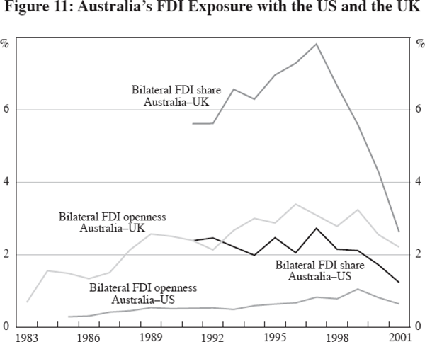
A different avenue might be to use bilateral FDI, however, reliable data are at best available only from the mid 1980s. Figure 11 shows bilateral indices for FDI similar to those we constructed for trade exposure for the UK and the US. Bilateral FDI openness measures the stock of bilateral FDI (inward and outward) as a share of GDP of both economies. The bilateral FDI share measures bilateral direct investment as a share of total FDI of both economies. Even though these are very short time series, the two measures do not necessarily give the same picture since the 1980s. FDI openness has risen overall, suggesting that bilateral FDI has grown at a faster pace than GDP. However, for these country pairings, total FDI has grown at an even faster pace than bilateral FDI, leading to falling bilateral FDI shares. This is not surprising since these economies are likely to have taken up other FDI opportunities, for example in China or east Asia. This is likely to dampen any measurable effect of bilateral FDI on the business cycle, since at the same time there would be spillovers from financial investments in these other (Asian) economies. Ultimately, more data and longer time series are required to assess any such effect.
4. Conclusions
Over the past 40 years, the Australian business cycle has become highly correlated with that of Canada, the UK, and the US. On the other hand, Australia's business cycle has become less correlated with that of Japan and the euro area. While previous studies have sought to explain business cycle correlations in a cross-country context, less is known about the factors which have caused these relationships to change so dramatically through time.
The results from this paper suggest that there is no single model that can explain changes in cycle co-movements across all the five economy pairs considered. However, many of the cross-sectional explanations for business cycle co-movements are also useful for explaining changes through time. For instance, the well-documented increase in Australia's business cycle correlation with the US could be at least partly explained by more similar industrial structures, which – in the presence of global industry-specific shocks – leads to more cyclical co-movement. Once we control for this effect, we find that the falling trade share with the US is likely to have had a dampening effect on cycle correlation.
For other economy pairings, however, the explanation suggested by our models is somewhat different. While the two most prominent variables from the cross-section literature – trade and industrial structure – are necessary to obtain a valid model, they are not sufficient. A move towards more similar degrees of labour market flexibility has a positive effect on cycle co-movement for our economy pairs, though the direction of this relationship is theoretically ambiguous, and is contingent on the nature of the shocks that prevail over the sample period. We also find evidence that for individual economy pairs where one economy has experienced a large idiosyncratic shock, such as for Japan and the euro area, measures of divergences in fiscal and monetary policy matter, possibly because they can capture some of this shock.
However, our models are likely to overstate the importance of individual factors, such as industrial structure, if these coincide with other factors omitted in our analysis. Monetary and fiscal policy are only one example where changes in shocks can affect cyclical co-movement. More generally, change in the nature of shocks that an economy pair is exposed to can alter business cycle co-movements. A thorough analysis of this is, unfortunately, beyond the scope of this paper.
Finally, we have also neglected some possible channels of transmission of shocks across countries. Despite our findings vis-à-vis trade, which has reduced business cycle co-movement across our economy pairs, we have not discounted the significance of increasing international economic interdependence. One would expect that closer financial market integration also plays a role, although the theoretical link is less clear. Limited data availability makes this a difficult hypothesis to test.
Appendix A: Data
Real GDP:
Quarterly real GDP data for Australia come from the Australian Bureau of Statistics (ABS), Cat No. 5206.0 for 1960:Q1 to 2004:Q4; for the euro area from Fagan, Henry and Mestre (2001) for 1970:Q1 to 1990:Q4, spliced to data from Eurostat (EMU-11 plus Greece) for 1991:Q1 to 2004:Q4; for New Zealand from Buckle, Haugh and Thomson (2001) for 1977:Q1:1987:Q1, spliced to data from Thomson Financial for 1987:Q2 to 2004:Q4; for all other countries from Thomson Financial for 1960:Q1 to 2004:Q4 (1961:Q1 to 2004:Q4 for Canada).
Trade measures:
Annual bilateral trade data (exports plus imports) for goods come from the Direction of Trade Statistics (IMF) for all countries from 1963, or earliest available. Data for the euro area were obtained by adding EMU member country figures and splicing backwards with average growth rates where individual smaller countries are unavailable. Since exports from country i to country j do not always equal imports recorded by country j, we have averaged these. Where only data from one country are available, we spliced backwards for the partner country using that series. Annual data were converted into quarterly data by linear interpolation.
Annual trade data vis-à-vis the world come from the same source as the bilateral trade data. Euro area data were calculated net of intra-EMU trade.
Quarterly nominal GDP comes from the same sources as real nominal GDP, except for New Zealand where data on GDP(P) for 1970:Q1 to 1987:Q1 were obtained from the RBNZ, spliced to data from Thomson Financial thereafter. These were converted into US$ using quarterly average exchange rates from the RBA.
Industrial structure:
Annual data for gross value added at constant prices by industry classification (ISIC) were compiled using a number of sources: the OECD International Sectoral Database (ISDB) and the OECD National Accounts II formed the basis. Updates for Australia used ABS data (Cat No 5204.0), prior to 1969 we used growth rates of employment by industry from the ISDB; for the UK we used O'Mahony (1999) to provide data for earlier years, and shares to calculate the weights (UK data are only available as index series) were obtained using current price series for the base year 1995, with updates from Thomson Financial; the euro area data were proxied with data from Germany and France for which earlier observations were provided by O'Mahony (1999), weighted using all industries gross value added; for the US we used data by the Bureau of Economic Analysis from 1987, which we matched with ISIC1 categories, and OECD and O'Mahony for data prior to 1987; data for New Zealand come from Buckle et al (2001); data for Canada come from Thomson Financial from 1981 and the Bank of Canada prior to 1981. Quarterly frequency for the dissimilarity index was obtained by linear interpolation.
Labour market flexibility:
Annual data on net union density come from Nickell and Nunziata (2001). Updates come from national sources and the ILO. The euro area data comprise Belgium, Finland, France, Germany, Italy, Netherlands, and Spain, weighted by euro-area weights as documented in Fagan et al (2001). Quarterly frequency for the dissimilarity index was obtained by linear interpolation.
Product market flexibility:
Index compiled by Nicoletti et al (2001) from a range of underlying indicators. Data are available every four to five years from 1978 to 1998. The euro-area data comprise Belgium, Finland, France, Germany, Italy, Netherlands, and Spain, and were aggregated using the euro-area weights of the individual countries employed by Fagan et al (2001).
Monetary policy:
Quarterly short-term interest rates (3-month maturity) come from Global Financial Data and Thomson Financial.
Fiscal policy:
Quarterly data on primary budget deficits for 1965:Q1 (or earliest available) to 2004:Q4, cyclically unadjusted as calculated by the OECD, come from Thomson Financial. For the euro area we sum the OECD data for Austria, Finland, France, Germany, Ireland, Italy and the Netherlands after 1996:Q1, and splice this to the data from Fagan et al (2001). Nominal GDP data are the same as for the trade measures.
Bilateral FDI:
Data on bilateral FDI stocks (inwards and outwards) come from the ABS Cat No 5302.0 (since 1990) and from the OECD foreign direct investment database (prior to 1990). Data on total FDI (assets and liabilities outstanding), as calculated in the International Financial Statistics, come from Thomson Financial.
Appendix B: Additional Figures
Footnotes
We would like to thank Anthony Rossiter, Amanda Armstrong, Bob Buckle, Graham Howard and Maximilian Layton for invaluable help with the data, and Luca Benati for sharing his Matlab code. Don Harding, Christopher Kent, Glenn Otto, Adrian Pagan, colleagues at the RBA and participants at the RBA annual conference 2005 provided valuable comments. [1]
See, for example, de Brouwer and Romalis (1996), de Roos and Russell (1996), Debelle and Preston (1995), Dungey and Pagan (2000), Gruen and Shuetrim (1994) and Otto, Voss and Willard (2001). [2]
Unless otherwise stated, sources for data underlying the tables or figures in this paper are authors' calculations. Details of the calculations and the source of the underlying data can be found in Appendix A. [3]
Shortening the window tends to result in a more volatile measure of business cycle correlation, which in the extreme case of the length of one business cycle can move between 1 and −1, depending on the phase shift between the cycles of the two economies. [4]
The band-pass filter of Baxter and King extracts the cyclical frequencies between 6 and 32 quarters, which coincides with the timing of cycles used in the seminal work on classical business cycles by Burns and Mitchell (1946). Since the filter incorporates a moving average, we lose three years of data at the beginning and at the end of the sample. The changes in co-movements through time are very similar if we use other filtering methods, such as the Hodrick-Prescott filter or the band-pass filter proposed by Christiano and Fitzgerald (2003), although the levels using the latter are lower for some of the country pairs. Gillitzer, Kearns and Richards (this volume) show that the change in the cycle co-movement between Australia and the US is also evident using cyclical measures other than GDP. [5]
Interestingly, the cycle correlation between Japan and the euro area has been between 0.6 and 0.8 over most of the sample, with the higher values of 0.8 being reached in the earlier part of the sample. [6]
However, as Kehoe (2005) notes, trade can only explain a very small fraction of cycle co-movement in their model, possibly a result of the large, heterogeneous sample of countries used. [7]
All our bilateral trade data are based on goods trade only, as bilateral services trade data are only available for a shorter period. [8]
Since, in the econometric section of the paper, we investigate only country pairings which involve Australia and larger trading partners, we can restrict ourselves to this simple choice. In a more systematic analysis, a decision rule that chooses the larger share would have to be applied, similar to that used by Otto et al (2001). [9]
For Figures 5 to 10 we have scaled the industrial dissimilarity index to lie between 0 and 200. More detailed sectoral breakdowns than ISIC1 have been used in the literature, but we are constrained by the requirement of data comparability across countries and over time. [10]
The ratio of the two indices can capture not only whether two economies have become more similar, but also which economy has become more flexible relative to the other. This allows us to compare it with other measures of flexibility. The absolute difference is used for the regressions. In our country pairings, these two measures give somewhat different profiles for Australia–UK, Australia–New Zealand and, to a lesser extent, Australia–Canada, where the indices cross each other over time. [11]
Initially we also considered a similar measure for 10-year bond interest rates, but we found that the profile over time did not differ substantially from that of 3-month interest rate differences. [12]
Due to limited data availability, we had to proxy some of the euro area data with data from Germany and France. Data are quarterly or annual, except for the product market index which is only available on a five-yearly basis and for a much shorter time period. It is therefore only included to allow for an approximate comparison. [13]
In fact, sectoral shares for Australia and the US have become more similar for most industries. One notable exception is the share of ‘financial services’, which increased markedly in both economies but by much more in Australia. [14]
It is not surprising that most of our economies had falling trade exposure with Australia, since over the last 20 to 30 years industrialised countries' trade has been increasingly oriented towards east-Asian economies and China. [15]
Integration tests confirm that all variables are I(0) or I(1). One could argue that, strictly speaking, a correlation coefficient is a summary statistic of a distribution, and therefore statistical concepts such as non-stationarity are misplaced. Moreover rolling correlation coefficients imply changing distributions. We share some of these conceptual problems with studies using rolling standard deviations of output, such as Barrell and Gottschalk (2004). An entirely different approach to our empirical problem would be to model the covariance and variance of two GDP cycles, conditional on exogenous factors. These could then be combined to estimate the impact on the correlation coefficient. We would like to thank Adrian Pagan for suggesting this alternative approach which we aim to evaluate in future research. [16]
Unfortunately, we do not have enough data to account explicitly for a full lag structure of 16 years, the length of our moving window. We have checked the robustness of our results by estimating a long-run model that explicitly takes account of an MA-error structure with 16 lags (that is, four years). For all models the results are very close to our DOLS regressions, and for almost all models only the first 6 to 8 lags are significant. [17]
We should point out that the inclusion of these variables implies also a shortening of the estimation period for these three economy pairs, since the fiscal policy variable is only available from 1970:Q1 and the monetary policy variable for Japan is only available from 1969:Q1. For the UK and Japan, this shortening is not material: over the shorter estimation period the policy variables are required to obtain co-integration. For Canada, however, we can obtain co-integration (at a 5 per cent significance level) over the shorter period without including fiscal policy. This is because our model has difficulties explaining the steep increase in correlation between 1963 and 1970. The coefficient estimates are only slightly affected by the inclusion of fiscal policy. [18]
The significance level of these coefficients should be treated with caution, as we may not have fully corrected for serial correlation in our model. [19]
We should note that for Canada, if fiscal policy and labour market flexibility are included, we have a co-integrating relationship where trade has a negative coefficient. However, the coefficient on labour market flexibility is not significant, and, once dropped, trade becomes positive, pointing to a problem of multicollinearity between trade and labour market flexibility. [20]
In our models, trade appears to be the most important factor in explaining the synchronicity changes with Japan and the UK (the latter with a negative sign), while industrial structure plays a larger role for Canada, the euro area and the US. The exact contribution varies with the model estimated. The results in Table 3 allow us to gauge the contributions from various factors to the estimated long-run changes in business cycle changes, but not for the actual changes since our model has a dynamic specification. Moreover, a variable which moves cyclically might be an important variable for the model although its overall contribution in explaining a (monotonic) trend might be small. [21]
We have also checked whether there is a role for fiscal or monetary policy, or both, in the other models. For Canada, the addition of monetary policy does not alter any of our results, and co-integration is somewhat less likely. For the euro area, we can include either policy variable or both, but the monetary policy variable affects other coefficients more strongly. For the UK, the inclusion of monetary policy does not alter anything. For Japan, we cannot find co-integration when we include fiscal policy. [22]
Of course, optimal portfolio allocation theory would suggest that, if one market has a low or negative return, investment should be shifted to the market with the higher return, rather than spending reigned in on all investments. [23]
References
Barrell R and S Gottschalk (2004), ‘The volatility of the output gap in the G7’, National Institute Economic Review, 188, pp 100–107.
Baxter M and RG King (1999), ‘Measuring business cycles: approximate band-pass filters for economic time series’, Review of Economics and Statistics, 81(4), pp 575–593.
Baxter M and MA Kouparitsas (2005), ‘Determinants of business cycle comovement: a robust analysis’, Journal of Monetary Economics, 52(1), pp 113–157.
Bayoumi T and B Eichengreen (1993), ‘Shocking aspects of European Monetary Union’, in F Torres and F Giavazzi (eds), Adjustment and growth in the European Monetary Union, Cambridge University Press, Cambridge, pp 193–229.
Blanchard OJ and J Wolfers (2000), ‘The role of shocks and institutions in the rise of European unemployment: the aggregate evidence’, Economic Journal, 110(462), pp C1–C33.
Bordo MD and T Helbling (2003), ‘Have national business cycles become more synchronized?’, NBER Working Paper No 10130.
Buckle RA, D Haugh and P Thomson (2001), ‘Calm after the storm?: Supply-side contributions to New Zealand's GDP volatility decline’, New Zealand Treasury Working Paper No 01/33.
Burns AF and WC Mitchell (1946), Measuring business cycles, NBER, New York.
Christiano LJ and TJ Fitzgerald (2003), ‘The band-pass filter’, International Economic Review, 44(2), pp 435–465.
Clark TE and K Shin (2000), ‘The sources of fluctuations within and across countries’, in GD Hess and E van Wincoop (eds), Intranational macroeconomics, Cambridge University Press, Cambridge, pp 187–217.
Clark TE and E van Wincoop (2001), ‘Borders and business cycles’, Journal of International Economics, 55(1), pp 59–85.
de Brouwer G and J Romalis (1996), ‘External influences on output: an industry analysis’, Reserve Bank of Australia Research Discussion Paper No 9612.
de Roos N and B Russell (1996), ‘Towards an understanding of Australia's co-movement with foreign business cycles’, Reserve Bank of Australia Research Discussion Paper No 9607.
Debelle G and B Preston (1995), ‘Consumption, investment and international linkages’, Reserve Bank of Australia Research Discussion Paper No 9512.
Dungey M and A Pagan (2000), ‘A structural VAR model of the Australian economy’, Economic Record, 76(235), pp 321–342.
Ebell M and C Haefke (2003), ‘Product market deregulation and labor market outcomes’, Swiss National Bank, Study Center Gerzensee Working Paper No 02.08.
Fagan G, J Henry and R Mestre (2001), ‘An area-wide model (AWM) for the euro area’, European Central Bank Working Paper No 42.
Forbes KJ and MD Chinn (2003), ‘A decomposition of global linkages in financial markets over time’, NBER Working Paper No 9555.
Frankel JA and AK Rose (1998), ‘The endogeneity of the optimum currency area criteria’, Economic Journal, 108(449), pp 1009–1025.
Funke M, S Hall and R Ruhwedel (1999), ‘Shock hunting: the relative importance of industry-specific, region-specific and aggregate shocks in the OECD countries’, The Manchester School Supplement, pp 49–65.
Gruen D and G Shuetrim (1994), ‘Internationalisation and the macroeconomy’, in P Lowe and J Dwyer (eds), International integration of the Australian economy, Proceedings of a Conference, Reserve Bank of Australia, Sydney, pp 309–363.
Heathcote J and F Perri (2002), ‘Financial globalization and real regionalization’, NBER Working Paper No 9292.
Imbs J (1999), ‘Co-fluctuations’, Centre for Economic Policy Research Discussion Paper No 2267.
Imbs J (2000), ‘Sectors and the OECD business cycle’, CEPR Discussion Paper DP2473.
Imbs J (2004), ‘The real effects of financial integration’, London Business School, mimeo.
Kalemli-Ozcan S, BE Sørensen and O Yosha (2001), ‘Economic integration, industrial specialization, and the asymmetry of macroeconomic fluctuations’, Journal of International Economics, 55(1), pp 107–137.
Kalemli-Ozcan S, BE Sørensen and O Yosha (2003), ‘Risk sharing and industrial specialization: regional and international evidence’, American Economic Review, 93(3), pp 903–918.
Kehoe P (2005), ‘Comment on “Determinants of business cycle comovement: a robust analysis&dsquo;’, Journal of Monetary Economics, 52(1), pp 159–162.
Kose MA, ES Prasad and ME Terrones (2003), ‘How does globalization affect the synchronization of business cycles?’, American Economic Review, Papers and Proceedings, 93(2), pp 57–62.
Krugman P (1991), Geography and trade, MIT Press, Cambridge.
Krugman P (1993), ‘Lessons of Massachusetts for EMU’, in F Torres and F Giavazzi (eds), Adjustment and growth in the European Monetary Union, Cambridge University Press, Cambridge, pp 241–269.
Kwark N-S (1999), ‘Sources of international business fluctuations: country-specific shocks or worldwide shocks?’, Journal of International Economics, 48(2), pp 367–385.
MacKinnon JG (1991), ‘Critical values for cointegration tests’, in RF Engle and CWJ Granger (eds), Long-run economic relationships, Oxford University Press, Oxford, pp 267–276.
Nickell S and L Nunziata (2001), ‘Labour market institutions database’, Centre for Economic Performance, London School of Economics, mimeo.
Nicoletti G, A Bassanini, E Ernst, S Jean, P Santiago and P Swaim (2001), ‘Product and labour markets interactions in OECD countries’, OECD Economics Department Working Paper No 312.
O'Mahony M (1999), Britain's relative productivity performance 1950–1996: an international perspective, National Institute of Economic and Social Research, London.
Otto G, G Voss and L Willard (2001), ‘Understanding OECD output correlations’, Reserve Bank of Australia Research Discussion Paper No 2001-05.
Otto G, G Voss and L Willard (2003), ‘A cross section study of the international transmission of business cycles’, University of Victoria, Canada, mimeo.