RBA Annual Conference – 2009 Global Relative Price Shocks: The Role of Macroeconomic Policies Adam Cagliarini and Warwick McKibbin [1]
Abstract
We use the multi-sector and multi-country G-Cubed model to explore the potential role of three major shocks – to productivity, risk premia and US monetary policy – to explain the large movements in relative prices between 2002 and 2008. We find that productivity shocks were major drivers of relative price movements, while shocks to risk premia and US monetary policy contributed temporarily to some of the relative price dispersions we observe in the data. The effect of US monetary policy shocks on relative prices was most pronounced in countries that fix their currency to the US dollar. Those countries that float were largely shielded from these effects. We conclude that the shocks we consider cannot fully capture the magnitude of the relative price movements over this period, suggesting that other driving forces could also be responsible, including those outside of the model.
1. Introduction
Between 2002 and 2008, the world experienced a very large shift in the prices of resources and commodities relative to other goods and services. For instance, between their trough in December 2003 and their peak in December 2008, resource export prices for Australia rose on average by 26 per cent annually in Australian dollar terms. Over the same period, prices for Australia's manufactured, agricultural and service exports rose on average by 2.7, 6.2 and 3.5 per cent annually. The IMF indices for primary commodity prices also imply significant relative price movements – relative to non-durable manufactured goods, energy prices almost tripled and agricultural prices rose by more than 50 per cent (Figures 1 and 2).
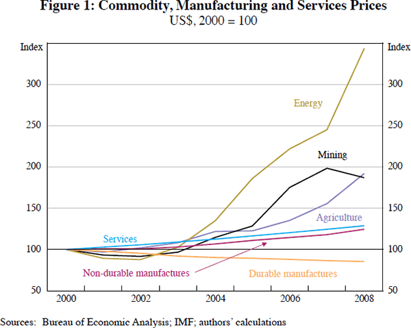
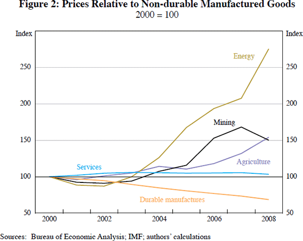
We explore the likely key drivers of these relative price movements by applying a range of shocks to the multi-sector, multi-country G-Cubed model. The goal is to improve our understanding of how major shocks are transmitted to inflation and changes in relative prices in different economies. These shocks include stronger productivity growth, particularly in manufacturing in developing economies (especially China), and an investment boom due to a reduction in risk premia globally. We also explore the role that monetary policies, particularly in China and the United States, may have had in driving these movements in relative prices. We then combine the various shocks and explore whether they are able to explain the global experience between 2002 and 2007.
2. The Role of Developing Economies
During the 1990s and 2000s, much of east and south-east Asia experienced a prolonged period of strong economic growth spurred by growth in productivity. The adoption of production processes from more developed economies helped to boost productivity levels of the economies in this region, while growth in investment helped to boost labour productivity. According to the IMF, labour productivity in Asia grew on average by 3.3 per cent per year between 1970 and 2005, of which capital accumulation contributed about 2 percentage points and total factor productivity (TFP) growth contributed 0.9 percentage points. Since 1979, labour productivity in China has grown by around 6 per cent annually (Table 1). TFP growth is estimated to account for half this growth while capital accumulation accounts for a significant proportion. Estimates of average annual TFP growth in China's manufacturing sector are as high as 10.5 per cent since 1998.[2]
| Start date | Labour productivity |
Physical capital |
Human capital |
TFP | |
|---|---|---|---|---|---|
| Japan | 1955 | 3.1 | 2.0 | 0.4 | 0.7 |
| NIEs | 1967 | 4.5 | 2.6 | 0.6 | 1.5 |
| ASEAN-4 | 1973 | 2.8 | 1.6 | 0.9 | 0.0 |
| China | 1979 | 6.1 | 3.0 | 0.9 | 3.6 |
| India | 1982 | 2.7 | 1.4 | 0.8 | 1.7 |
| Other Asia | 1990 | 2.6 | 1.3 | 0.8 | 0.4 |
|
Notes: NIEs (newly industrialised economies) consists of Hong Kong SAR, Singapore, South Korea and Taiwan Province of China. ASEAN-4 consists of Indonesia, Malaysia, the Philippines and Thailand. Source: IMF (2006) |
|||||
While growth in productivity has had direct effects on relative prices, particularly on the goods that Asian economies export, the effects on relative prices have not solely been driven by supply-side factors. In particular, the increase in productivity sparked an investment boom in these economies, and economies that industrialise increase their demand for resources. Accordingly, the energy needs of Asia increased significantly. China, which by 2007 accounted for about 7.5 per cent of global energy consumption, was responsible for nearly 50 per cent of the growth in global energy consumption between 2000 and 2007, while the rest of the Asia-Pacific region accounted for 18 per cent of growth in world energy consumption (see BP 2008). In comparison, North America was responsible for only 5 per cent of the growth in global energy consumption. The effect of the increased demand for resource commodities, as well as the downward pressure on prices for manufactured goods that Asia produces and exports, were major contributors to the large relative price movements.
Of course, changes in relative productivity levels, taxes and shifts in consumer preferences may also affect relative prices. However, the trends in relative prices, such as we have seen in the past decade, have also been driven by demand for certain goods from countries at earlier stages of their economic development. China and India have had the effect of increasing demand for certain commodities, especially energy and mineral products, while the prices of the products they export, for which they have a comparative advantage, have not risen by as much and in some cases have fallen.
3. Monetary Policies around the World
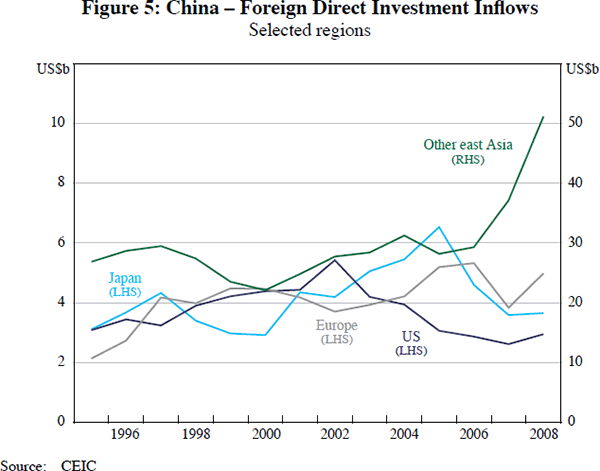
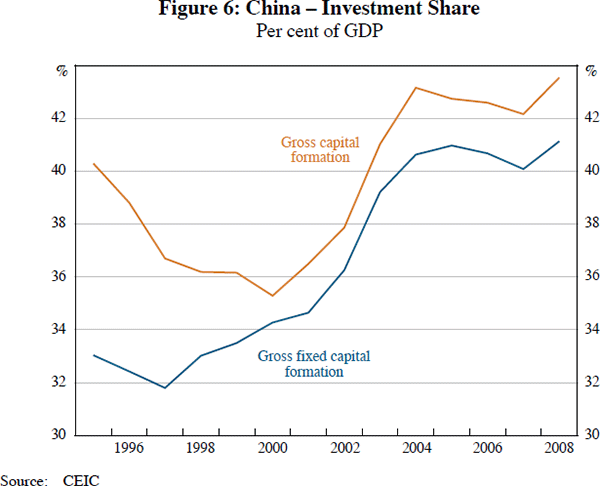
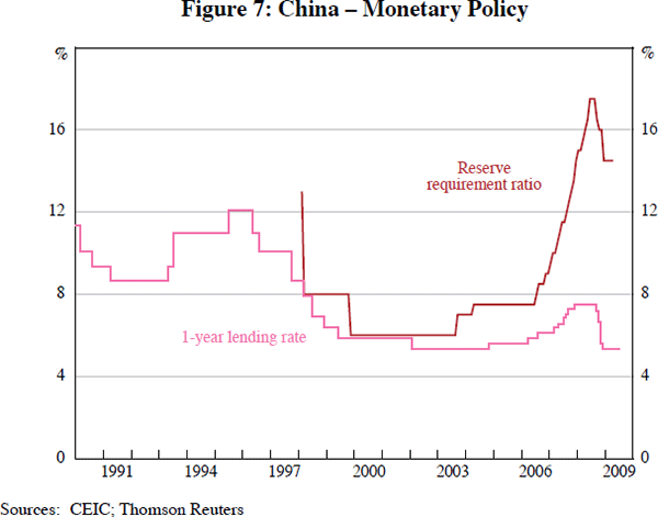
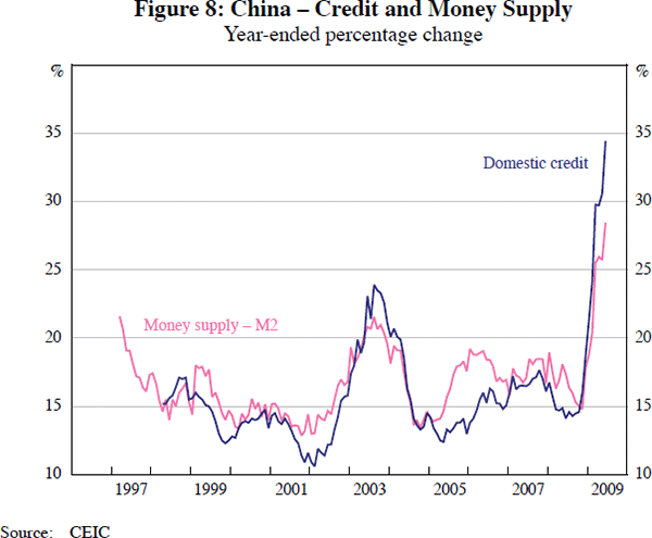
To some extent, the dramatic changes in relative prices could be the result of a combination of monetary policies adopted in the United States, China and elsewhere in the world. Following the events of 11 September 2001, the bursting of the dot-com bubble and at the onset of the 2001–2002 recession, the Federal Reserve Board (FRB) lowered interest rates aggressively, only gradually increasing rates as the US economy recovered (Figure 3). By fixing its exchange rate to the US dollar for a prolonged period of time after devaluing its currency in 1993 (Figure 4), China substantially reduced exchange rate risk for investors. The fixed exchange rate regime adopted by China, combined with the large interest rate differential that resulted from China not adjusting its interest rates to the same extent as the United States, encouraged firms to borrow in US dollars to invest in China, receiving higher returns with little fear of a devaluation of the Chinese currency. This is evident in the rapid growth of the gross flow of foreign direct investment into China, from US$47 billion in 2001 to US$108 billion in 2008, driven mainly by firms domiciled in east Asia, particularly from Hong Kong (Figure 5). Also, China's foreign exchange reserves grew exponentially – foreign reserves by July 2009 were about US$2.1 trillion, 10 times their level at the beginning of 2002 (Figure 4) – and gross fixed capital formation as a share of GDP rose quite rapidly in China (Figure 6). This boom in investment led directly to increased demand for raw materials and a large increase in commodity prices, particularly energy prices. Even as China increased interest rates and used other tools to tighten monetary policy, such as increasing its reserve requirement ratio (Figure 7), investment remained high and foreign direct investment rose rapidly. While the increase in the reserve requirement ratio acted to restrict lending by banks in China (Figure 8), it did not stop firms reinvesting their profits nor did it slow the inflow of foreign direct investment.
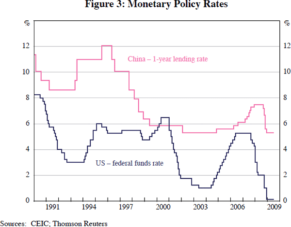
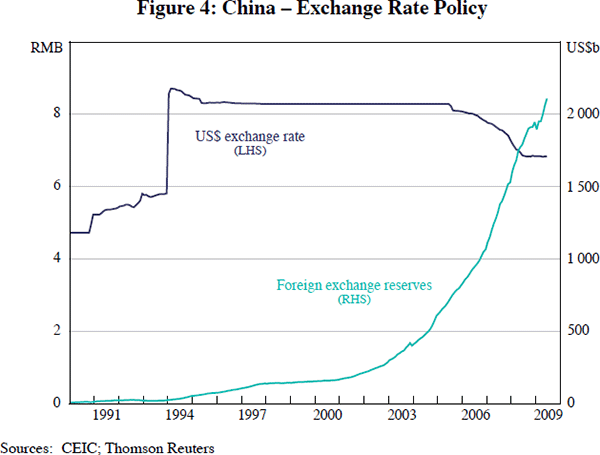
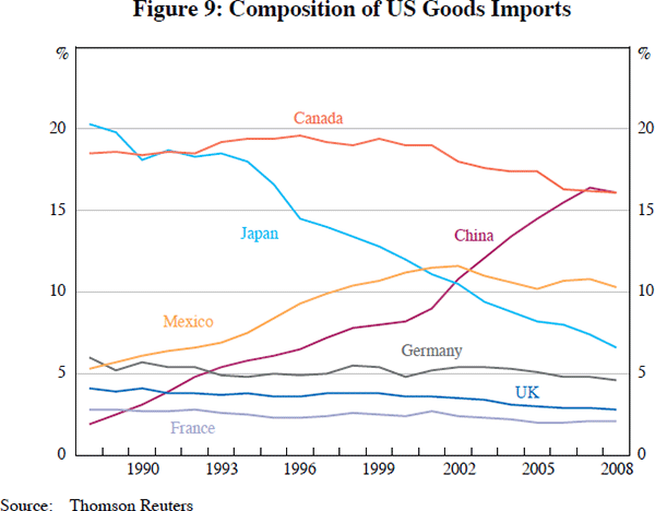
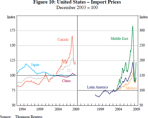
Import prices from countries such as China clearly exerted some downward pressure on US inflation. Although some have argued that US monetary policy was too easy between 2002 and 2006, it is difficult to argue that US monetary policy alone was behind the large movement in relative prices. The United States, during this period, was increasing its imports from China, to the point where China was close to becoming the largest source of US imports (Figure 9). This was the result of the lower prices of goods imported from China, mainly at the expense of imports from Mexico. The resulting downward pressure on inflation enabled the FRB to keep nominal interest rates reasonably low without risking rising inflation for prices of goods and services. Conversely, import prices from commodity-producing countries were rising rapidly (Figure 10), although some of this movement, especially between the middle of 2005 and the middle of 2008, could be attributed to the depreciation of the US dollar. The price of imports from China began to rise in 2006 following China's move to revalue its currency against the US dollar.
In the remainder of this paper, we apply a sequence of shocks to the multi-sector global G-Cubed model to see the extent to which the relative price movements that were observed across six different sectors can be replicated. The six sectors are: agriculture, mining, energy, durable manufactures, non-durable manufactures and services. Although the model contains many economies, we focus on just three: the United States, China and Australia. The shocks we consider are those to productivity, risk premia and monetary policy. We use these shocks to approximate some of the key features of the data, namely the large relative price movements and the boom in investment, particularly in China and other developing economies.
4. The Model
G-Cubed is a widely used dynamic intertemporal general equilibrium model of the world economy (which can be thought of as a hybrid dynamic stochastic general equilibrium (DSGE) model).[3] In the version used in this paper, there are 15 regions (Table 2), each with six sectors of production. The model produces annual results for trajectories running decades into the future.
| United States | China |
|---|---|
| Japan | India |
| United Kingdom | Other Asia |
| Germany | Latin America |
| Rest of euro area | Other LDC (less developed countries) |
| Canada | Eastern Europe & former Soviet Union |
| Australia | OPEC |
| Rest of the OECD |
Because G-Cubed is an intertemporal model, it is necessary to calculate a baseline, or ‘business-as-usual’ solution before the model can be used for policy simulations. In order to do so, we begin by making assumptions about the future course of key exogenous variables. We take the underlying long-run rate of world population growth plus productivity growth to be 1.8 per cent per year, and take the long-run real interest rate to be 4 per cent. We also assume that tax rates and the shares of government spending devoted to each commodity remain unchanged.
In the G-Cubed model, projections are made based on a range of input assumptions. There are two key inputs into the growth rate of each sector in the model. The first is the economy-wide population projection, which differs by economy according to the mid-projections made by the United Nations.[4] The second is the sectoral productivity growth rate. For the baseline, we follow McKibbin, Pearce and Stegman (2007), where each energy sector in the United States is assumed to have a rate of productivity growth of 0.1 per cent over the next century. Each non-energy sector has an initial productivity growth rate close to historical experience but gradually converging to 1.8 per cent per year in the long run. We then assume that each equivalent sector in each of the other economies will catch up to the US sector in terms of productivity, closing the gap by 2 per cent per year, except for developing countries, which are assumed to close the gap by 1 per cent per year. The initial gaps are therefore critical for the subsequent sectoral productivity growth rate. We assume that the initial gap between all sectors and the US sectors are equal to the gap between aggregate purchasing-power-parity (PPP) GDP per capita between each economy and the United States. We cannot easily use sectoral PPP gap measures because these are difficult to get in a consistent manner and with a sufficient coverage for our purposes. Thus the initial benchmark is based on the same gap for each sector as the initial gap for the economy as a whole. If we then have evidence that a particular sector is likely to be closer to, or further away from, the US sectors than the aggregate numbers suggest, we adjust the initial sectoral gaps while attempting to keep the aggregate gaps consistent with the GDP per capita gaps.
Given these exogenous inputs for population growth and the growth of productivity across sectors, we then solve the model with the other drivers of growth, namely capital accumulation and sectoral demand for inputs of energy and other materials, which are all endogenously determined. Critical to the nature and scale of growth across economies are the assumptions outlined above plus the underlying assumptions that: financial capital flows to where the return is highest; physical capital is sector-specific in the short run; labour can flow freely across sectors within a country but not between economies; and international trade in goods and financial capital is possible, subject to existing tax structures and trade restrictions. Thus the economic growth of any particular economy is not completely determined by the exogenous inputs in that country alone, since all countries are linked through goods and asset markets.
In the analysis in this paper, we start with a projection of the model from 2002 onwards assuming steady-state growth in productivity as described above. We impose each shock, generate results in terms of deviations from the baseline and thereby determine the contribution of each shock to changes in relative prices and macroeconomic variables.
4.1 Policy responses
The results of this exercise will depend on the monetary and fiscal reactions. We assume that fiscal deficits are not changed in these results so as to focus on the core shocks without any fiscal stabilisers; that is, any changes in revenue are offset by changes in government spending spread across sectors based on historical spending shares. Of course, alternative assumptions regarding fiscal policy will change the results. The monetary responses have each economy following a Henderson-McKibbin-Taylor (HMT) rule shown in Equation (1), with different weights on inflation (π) relative to target (πT), output growth (Δy) relative to potential growth (ΔyT) and the change in the exchange rate (Δe) relative to target (ΔeT).

The assumed parameter values are set out in Table 3. Note that China and most developing economies have a non-zero weight on the change in their exchange rate relative to the US dollar.
| Economy | Inflation (β1) |
Output growth (β2) |
US$ exchange rate (β3) |
|---|---|---|---|
| United States | 0.5 | 0.5 | 0 |
| Japan | 0.5 | 0.5 | 0 |
| United Kingdom | 0.5 | 0.5 | 0 |
| Germany(a) | 0.5 | 0.5 | 0 |
| Rest of euro area(a) | 0.5 | 0.5 | 0 |
| Canada | 0.5 | 0.5 | 0 |
| Australia | 0.5 | 0.5 | 0 |
| Rest of the OECD | 0.5 | 0.5 | 0 |
| China | 0.0 | 0.0 | −10,000 |
| India | 0.5 | 0.5 | −10 |
| Other Asia | 0.5 | 0.5 | −1 |
| Latin America | 0.5 | 0.5 | −1 |
| Other LDC | 0.5 | 0.5 | −1 |
| Eastern Europe & former Soviet Union | 0.5 | 0.5 | −1 |
| OPEC | 0.5 | 0.5 | −10 |
| (a) Germany and the rest of the euro area have a fixed exchange rate with each other with a common interest rate, inflation target and output growth target. | |||
5. The Shocks
A number of shocks to the model are considered and although the focus is on producing multipliers for the effect of each shock on inflation and relative price changes, the shocks are scaled in such as way as to be plausible and to give a crude indication of how much of the observed changes in relative prices from 2002 might be explained within the model.
We first consider a surge in productivity growth in both durable and non-durable manufacturing sectors in developing economies, particularly China. The assumption is that TFP growth in China rises above baseline for a decade before returning to baseline (that is, closing the now smaller gap with the United States at 2 per cent per year). The actual shocks are shown in Table 4; the other economies are scaled to the Chinese shocks as shown. We also set growth in energy, mining and agriculture productivity to zero so that supply shortages emerge gradually over time.
| Productivity growth rate | |
|---|---|
| Energy (all countries) | 0 forever (1.8% below trend) |
| Mining (all countries) | 0 forever (1.8% below trend) |
| Agriculture (all countries) | 0 forever (1.8% below trend) |
| Services (all countries) | Trend |
| Durable manufactures (LATC)(a) | |
| China | 12% above trend for 9 years |
| India | 6% above trend for 9 years |
| Other Asia | 6% above trend for 9 years |
| Latin America | 6% above trend for 9 years |
| Non-durable manufactures (LATC)(a) | |
| China | 12% above trend for 9 years |
| India | 6% above trend for 9 years |
| Other Asia | 6% above trend for 9 years |
| Latin America | 6% above trend for 9 years |
| Risk premia shock | |
| China (all sectors) | −10% forever |
| All other countries and sectors | −5% forever |
| (a) LATC = labour-augmenting technical change | |
The second shock is a fall in global risk, most notable for China, in the form of a reduction in equity risk premium in each sector. This leads to an investment boom in China and some other economies. The scale of the changes to risk premia are also shown in Table 4.
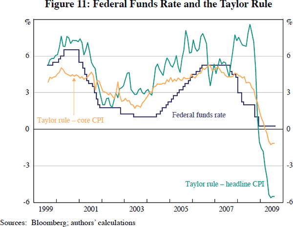
The third shock is to monetary policy over a number of years, with interest rates kept lower than otherwise. The logic for this is as follows. The Taylor rule (also known in the literature in a more general form as the HMT rule) is often used as a guide to measure the level of the short-term nominal interest rate. Between 2001 and 2006, the federal funds rate was below the rate implied by a widely used parameterisation of the Taylor rule by a significant margin (see Taylor 1993, 2009).[5] Using the core PCE measure of inflation, between June 2001 and January 2006, the federal funds rate was below the standard Taylor rule recommendation by an average of around 125 basis points (Figure 11). By this metric, monetary policy was very accommodative during this period. There are a number of ways of trying to engineer a path of interest rates that is below that recommended by some stylised rule. We could use additive shocks to generate a path for interest rates that deviates from the rule. Another way of generating this deviation is to argue that the FRB had assumed a higher growth rate for potential output, thereby lowering their estimation of the output gap leading to lower interest rate settings. Whatever the justification, the key point is that the shocks imply an interest rate path in line with those actually implemented by the FRB from 2001 to 2006.
The size of the shocks we incorporate seem reasonably plausible in light of actual developments over the past seven years or so. The key question then is whether, when combined in the model, they are sufficient to explain the movements of inflation and relative prices over this period. To the extent that the shocks might not be sufficient, other shocks may need to be incorporated into a further analysis, and/or the model may need to be modified in some way.
6. Results
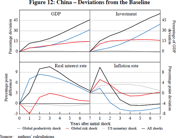
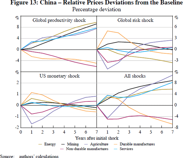
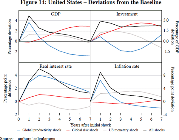
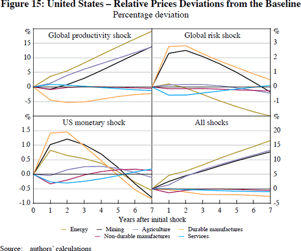
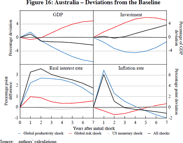
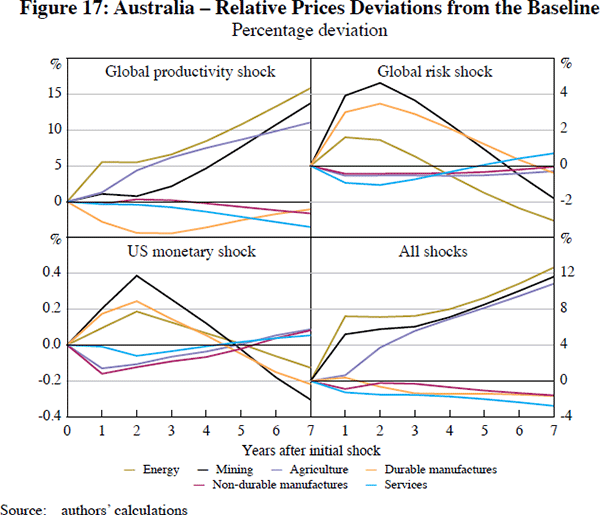
The results of each shock are shown in Figures 12 through 17. These figures display the deviations from the baseline of key variables. Figures 12 and 13 contain results for China, Figures 14 and 15 for the United States, and Figures 16 and 17 for Australia. The figures show the response to each of the three shocks (separately and combined) of: GDP; investment; the real interest rate; and inflation. The responses of prices for each of the six sectors in each economy (relative to the output price index of each economy) are also shown for the combination of the three shocks.
To understand the results it is important to note a key feature of the G-Cubed model. A good produced in a sector within a country is an imperfect substitute for the same good produced in the same sector in another country. Thus, although there are six sectors of production in each country, and each sector within each country has a similar name, in effect there are actually 90 different goods in the model (6 sectors times 15 economies). Every sector has the same production function in each economy, with the same elasticity of substitution between the factors of production. The initial input share coefficients are from recent input-output tables for each economy and differ across sectors and across economies.[6] Thus mining in China is initially relatively labour intensive whereas mining in Australia is relatively capital intensive.[7] Since the production technologies to produce investment goods, and goods and services consumed by governments and households have finite elasticities of substitution, there is never complete convergence in the production technologies of the sectors across economies.
6.1 Productivity shocks
First consider the effect of productivity shocks. The rise in manufacturing productivity in developing economies raises investment in the manufacturing sectors in those economies. The lack of growth in energy, mining and agriculture productivity worldwide tends to retard investment in those sectors. In China, the rise in productivity raises GDP growth and the level of GDP rises further above the baseline each year (Figure 12). Note that the results for GDP in each figure are shown as percentage deviations from the baseline in levels, while the productivity shock is to the growth rate of productivity. Higher productivity growth in manufacturing offsets the low productivity growth in non-manufacturing so that aggregate investment rises and the capital stock grows to the new higher level. Because the shock to the growth rate eventually disappears, the level of GDP and capital will remain permanently higher. Higher expected incomes in China raise consumption. Together with higher investment, aggregate demand temporarily rises above aggregate supply and inflation temporarily rises even though it falls over time. This latter effect follows because the higher growth in China implies that the real exchange rate needs to depreciate (since China has to sell more goods to the rest of the world). Since the nominal exchange rate is fixed, this real depreciation occurs via lower inflation in China (helped about by higher real interest rates).
The top-left panel of Figure 13 shows the relative price impacts of the shock to productivity for China. The sectors in which there is strong productivity growth (durable and non-durable manufactures) experience falling input costs and lower prices relative to the economy average. Sectors that are not growing quickly (energy, mining and agriculture) are in greater demand as inputs into manufacturing production but also for higher investment and consumption. Thus the relative prices of these sectors tend to rise as their output becomes increasingly scarce relative to that of the manufacturing sectors. The demand for services also increases as this is a major input into production and consumption. By year 7 the price of energy is 16 per cent higher than the price of non-durable manufactures.
There is an additional important effect on durable versus non-durable goods. A rise in real interest rates tends to reduce the demand for output of the sectors that are producing inputs into capital goods or for goods whose demand depends on the calculation of the present value of a flow of future services. This is particularly an issue for the durable goods sector since it is a large input into producing the investment good that is purchased by all sectors. At the same time, sectors that are relatively capital intensive experience a larger increase in the rental cost of capital and therefore will contract relative to labour-intensive sectors when the real interest rate rises relative to the real wage. In China, the durable goods and energy sectors are capital intensive. Mining is relatively labour intensive in China but relatively capital intensive in the United States and Australia.
The macroeconomic implications of the rise in developing country productivity for the United States are shown in Figure 14. US GDP rises as a result of the shock in the developing economies, with consumption rising due to higher income from investments in developing economies. However, the GDP increase is short-lived as capital flows from the United States into developing economies in response to higher returns to manufacturing in those economies and due to higher energy and mining prices in the world. The hollowing-out of US manufacturing implies that GDP is 2.5 per cent below baseline by year 7 even though the growth rate of US GDP has returned to its long-run steady state.[8] The restructuring of US manufacturing also drives the response of aggregate investment (panel 4, Figure 14). While there is additional investment in non-energy sectors, this is outweighed by the decline of manufacturing. The outflow of capital from the United States to developing econommies increases real interest rates in the United States, which further acts to reduce US investment. As for inflation, the initial strength of consumption in the United States, together with higher non-manufacturing prices, is sufficient to initially offset the lower price of imported manufactured goods. However by year 4, the productivity shock is deflationary for the United States.
The outcomes for relative prices in the United States are shown in the top left panel of Figure 15. The pattern is very similar to that in China, with the relative price of energy, mining and agriculture rising relative to manufacturing. Despite the manufacturing productivity shock occurring outside the United States, the fall in the relative price of manufactured goods by year 7 in the United States is larger than in China (22 versus 16 per cent respectively).[9] The one difference between the United States and China, apart from the scale of the response, is that the price of services rises in China whereas it is flat in the United States. This is because there is a larger rise in consumption and, particularly, investment in China, which raises the demand for services by more than in the United States.
The responses in Australia to the productivity shocks are shown in Figure 16 and the top left panel of Figure 17. The results for GDP are similar to the United States in the short run. However, over time the assumption of no productivity growth in the relatively large sectors of the Australia economy – energy, mining and agriculture – weigh heavily on the growth of overall GDP. The increase in the real interest rate also reflects the flow of capital out of Australia into developing economies' manufacturing sectors, but this effect is smaller than for the United States because there is an inflow of investment into mining for export to the rapidly growing developing economies, which are demanding more raw materials.
6.2 Global risk shocks
The reduction in global risk (larger in China than everywhere else) takes the form of a fall in the equity risk premium. The adjustment mechanism in the model occurs through a rise in Tobin's Q for investment in each sector. This causes an investment boom in all countries, especially in China where the shock is largest. As can be seen from the macroeconomic results for China (Figure 12), the United States (Figure 14) and Australia (Figure 16), the adjustment across economies is very similar and as expected. Strong investment raises GDP via short-run demand effects. Over the medium term, GDP rises with the level of potential output, in line with higher capital accumulation. However, there are some subtle differences across countries. In China, monetary policy targets the exchange rate. Whereas real interest rates rise in the United States and Australia – following the initial shock to demand – in China, real interest rates fall initially as otherwise the Chinese currency would tend to appreciate (given the larger decline in the equity risk premium there).
The sectoral story for the risk shock is very different to the results for the productivity shock. As discussed above, the changes in real interest rates relevant to firms and households have very different impacts across sectors depending on how sectoral output is used and on the capital-labour ratio of each sector. The fall in the interest rates faced by households and firms tends to increase the demand for capital-intensive goods, inputs into capital-intensive industries and durable goods. In all economies, the fall in risk premia causes a rise in the demand for durable manufacturing goods and a rise in the relative price of these goods.[10] Note that mining output rises slightly in China because despite being relatively labour intensive, it is a large input into durable goods production. In both the United States and Australia, where mining is relatively capital intensive, there is a rise in the relative price. Agriculture prices fall sharply in China because agriculture is relatively labour intensive whereas in the United States and Australia, services prices fall by most because they are relatively labour intensive. (Agriculture is more capital intensive in these economies than in China.)
Another interesting insight from the results is that the initial demand change determines the short-run relative price changes in the model. However, over time investment and movements of labour across sectors change the supply side of some sectors. Thus, the medium-term relative price changes reflect a combination of demand and supply effects. So although the price of durable goods increases most in the short run in China, this induces greater investment in durable goods, which expands the supply of these goods and by year 7, the relative price of durables has fallen below the output price index.
6.3 Monetary policy shock
The final shock we consider is to monetary policy with the FRB setting policy rates below those implied by a standard Taylor rule. It is useful to start the analysis with the results for the United States shown in Figure 14. The US real interest rate is 50 basis points lower than baseline initially, falling to 1 percentage point below baseline by year 5. This stimulates investment, which raises real GDP above trend for a number of years, but at the same time it pushes up inflation by 2.5 to 3 percentage points. The integral of the difference in real GDP over time is zero because the higher real GDP in the first six years is then followed by GDP below base in subsequent years (not shown).
It is interesting to observe that the change in US monetary policy does change relative prices in the short run (Figure 15). The channel of adjustment is through the impact of real interest rate changes on the demand for durable goods and investment, and depends on the capital intensity of production of different sectors (as discussed above). In year 1, inflation rises by almost 3 percentage points and the price of durable goods relative to non-durable goods rises by 1.7 per cent. As would be expected, this relative price adjustment is largely gone by year 5. The persistence partly reflects the investment changes which propagate a supply response well after the demand response has passed. Thus relative prices overshoot in subsequent years due to the capital accumulation dynamics.
Interestingly, and perhaps not surprisingly, the results for China are very similar to the results for the United States – given that China pegs its currency to the US dollar. Thus the real interest rate falls in China as US monetary policy is relaxed in order to hold the exchange rate fixed. It is difficult to see in Figure 12 because of the scale of the other shocks, but Chinese inflation rises by 3.5 per cent by year 3 as China imports the easier US monetary policy. Chinese real GDP is 1.3 per cent higher by year 2 due to the monetary expansion. Although not as large as the results for the productivity shocks in China, this effect is nonetheless significant. The dispersion of relative price changes in China is also similar to that for the United States and for the same reasons. The one difference again is the mining sector, which is relatively labour intensive in China and therefore does not receive as much stimulus as in the United States where it is relatively capital intensive.
From the results in Figure 16 and 17, it is clear that the floating exchange rate largely insulates the Australian economy from the change in US monetary policy. Real interest rates fall but the effect is small. Nonetheless there are changes in relative prices because of a minor capital intensity effect in Australia, which is due in part to the small change in Australian real interest rates, but more importantly because the United States and China are a large share of the global economy. The dispersion in US relative prices of 1.8 percentage points and in China of 2.7 percentage points is reflected in the dispersion in relative prices in Australia of 0.8 percentage points. The flexible exchange rate only offsets aggregate price relativities but has little influence on the relative price differences across sectors.
6.4 Combining the shocks
Each of the figures also contains the results of combining all of the shocks in order to get a rough sense of how they offset or reinforce each other. Several interesting insights emerge when compared to the actual experience since 2001. First, while the developing economy productivity shocks are deflationary, this effect is offset by the change in US monetary policy so inflation is largely unchanged in the United States. Hence, from this perspective, US monetary policy appears to have been successful given the announced concern at the time regarding the potential for US deflation after the dot-com bubble burst in 2001.
Second, although the relative prices of energy, mining and agriculture after seven years move in the same direction as that experienced in the world economy over the period 2002 to 2007, the magnitudes are far smaller than the actual experience. The extraordinary magnitudes of the relative price changes between 2005 and 2007 observed in the global economy are not captured by the shocks to fundamentals considered in this modelling exercise. The sharp rise in the relative prices of commodities in excess of the model simulations could be explained by three different causes: speculative activities not built into the analysis in this paper; a set of shocks not considered in this paper; or misspecification of the model (that is, the model may not adequately reflect reality).
7. Relative Prices and the Role of Policy
Although monetary policy may have had only a minor role in driving the trends in relative prices over the past decade, our simulations show that it is possible for monetary policy to have an effect on relative prices in the short to medium term. It is also possible that the decline in global risk premia up to 2007 as investors searched for yield was also driven, at least in part, by monetary policies globally, even though we assume it to be a separate shock in this paper. Although we do not formally explore the optimal policy responses to the shocks driving the large relative price movements that the world economy has experienced, it is worth discussing some of the principles that macroeconomic policies should follow in response to these forces.
The presence of nominal rigidities, affecting some wages and/or prices, and real rigidities, such as capital adjustment costs, make it possible for monetary policy to have some effect on relative prices, including the terms of trade and real exchange rates. In an economy with sticky wages or prices, an easing of monetary policy will result in prices that are more flexible rising faster than those that are more sticky. This leads to a temporary shift in demand towards the sticky-price sectors. As sticky prices gradually adjust, relative prices and output will eventually return to long-run equilibrium. In the meantime, given a temporary fall in real interest rates, demand for durable goods, for example, should expand faster than in other sectors. Accordingly, the prices of capital-intensive sectors should rise by more while real interest rates are low.
When and how monetary policy should respond to relative price movements will depend on the nature of the shocks driving these changes. If they are very temporary, there may be little if any time to respond given the lag with which monetary policy can take effect. If the shocks are more persistent (though still temporary), much of the literature would argue that there are circumstances under which it is optimal for policy-makers to essentially do nothing – that is, not to respond to the shocks driving relative prices and to tolerate the resulting deviation of inflation from a target for a short time so long as this does not jeopardise hitting the inflation target over the medium term. There are circumstances, however, when policy may want to actively respond so as to speed the transition to the new relative price equilibrium; along the way inflation may well deviate from target, so again, the monetary authorities will need to ensure that inflation remains anchored to the target over the medium term. Of course, in practice it is difficult for policy-makers to recognise in real time whether a shift in relative prices is being driven by temporary or permanent factors, nor can they be certain about the extent to which policy can successfully fine-tune a faster transition if required.
Aoki (2001) examines the optimal monetary policy responses to relative price changes in both a closed economy model and a small open economy model and draws similar conclusions to those presented here. The models are based around two sectors, one with flexible prices, the other with sticky prices. The main findings are that stabilising relative prices around their efficient level should be a goal of a central bank and that targeting inflation in the sticky-price sector is sufficient to achieve this goal. In an open economy context, Aoki argues that the central bank should target domestic inflation since imported prices are typically flexible. By targeting domestic inflation, the central bank can effectively keep the real exchange rate at its optimal level, which is desirable from a welfare perspective. The argument that central banks should try to stabilise relative prices around their efficient levels could be extended to a world with other distortions not resulting from nominal rigidities.
Benigno (2002) examines optimal policy in an open economy, sticky-price model. In a closed economy model, optimal monetary policy tends to be somewhat expansionary in order to offset the distortion implied by monopolistic competition. In an open economy setting, if monetary authorities behave non-cooperatively, there is another mechanism that works in the opposite direction. Each policy-maker aims to improve their terms of trade and to shift the burden of production to the other country by appreciating their currency in the presence of nominal rigidities. The incentive for such contractionary policy is greater the more open an economy and the more substitutable domestic and foreign goods are in consumption. Others, like Canzoneri and Henderson (1991), find a similar contractionary bias but for a different reason. In their one-shot, two-country game, tighter monetary policy in one country leads to a real depreciation and higher inflation for the other country. Hence, following a common shock that raises inflation in both economies, monetary authorities in both countries try to engineer a real exchange rate appreciation by tightening monetary policy. The result of this combined action by the two policy authorities in a non-cooperative Nash equilibrium is that monetary policy becomes excessively tight in both economies compared to an equilibrium when the policy actions in the two countries are coordinated.
While monetary policy can only have relatively temporary effects on relative prices[11], fiscal policy can have more enduring effects. The use of fiscal instruments to address permanent changes in relative prices, however, is not without its problems and policy-makers need to take some care when using spending and taxing instruments to effect a change in relative prices. Should the shift in relative prices be the result of reduced competition in a particular market, or distortions due to fiscal policies abroad, there may be a case for a government to levy taxes or provide subsidies to offset the effect of these other distortions on relative prices. However, if relative prices are changing due to more fundamental factors, such as a shift in relative productivity levels, a fiscal authority working to offset the resulting shift in relative prices will lower welfare by distorting the allocation of resources.
There are other questions related to how a fiscal authority should deal with the boom in revenues that may result from a large terms of trade boost. Countries whose industries are highly concentrated in the production of a few commodities that may experience large increases in their prices will need to manage revenues carefully. Should the price of a particular commodity rise temporarily, it would be prudent of fiscal authorities to invest the windfall in another economy. This way, the fiscal authority, whose revenues may already be sensitive to the domestic economic cycle, can diversify its revenue risk; should commodity prices fall, along with the economy's real and nominal exchange rates, the domestic currency value of the government's investments overseas will rise as a result. Examples of this type of fund, known as sovereign wealth funds, include Chile's Economic and Social Stabilization Fund and Norway's Government Pension Fund Global (a continuation of the Petroleum Fund). Ideally, these funds would be invested in sectors not related to the sources of the shifts in the price of the commodity in question.
8. Conclusions
This paper considers a stylised representation of three major shocks affecting the global economy during the period from 2002 to 2008. These shocks were: a large rise in the productivity growth of manufactures relative to non-manufacturing sectors in developing economies; a fall in global risk premia; and the relatively easy monetary policy stance of the FRB starting after the bursting of the dot-com bubble in 2001 and lasting up until the early part of 2006. The three shocks are considered in a global model that captures the interdependencies between economies at both the macroeconomic and sectoral levels.
There are a number of insights that suggest a need for further empirical analysis. The first is that the shift in relative prices observed since 2002 can be partly explained by the adjustment in the model in response to the assumed shocks, however, the scale of the actual rise in the prices of energy, mining and agriculture relative to manufacturing since 2004 are not well captured. Other factors outside the fundamentals in the model are needed to explain the scale of this more recent experience. The second insight is that the model suggests that there was some contribution to global inflation due to the FRB keeping interest rates low after the bursting of the dot-com bubble in 2001, and that this effect was reinforced by the fact that the Chinese and other monetary authorities pegged to the US dollar. However, the effect on global relative prices of US monetary policy is relatively small compared to the productivity shocks in developing economies. One interpretation of these results is that the short-term deflationary impact of developing economy productivity growth on the US economy was to a large extent neutralised in the United States by the change in FRB policy as modelled in this paper.
An interesting conclusion of the simulations in this paper is that monetary policy tends to affect relative prices for up to four years because the effect of a temporary change in real interest rates varies across sectors. The effect depends on each sector's relative capital intensity as well as on the change in the demand for the output of each sector as consumption and investment adjust. Eventually the effect of monetary policy on relative prices dissipates.
Interestingly, a country that pegs to the US dollar when the United States relaxes monetary policy inherits both the overall inflationary consequences of the US policy shift as well as the dispersion in relative prices, although this partly depends on the relative capital intensity of the sectors in the pegging economy. A country, such as Australia, which maintains a flexible exchange rate is largely shielded from the inflationary effect of changes in US monetary policy (via an appreciation of the exchange rate) but it is not shielded from the relative price effects. These are transmitted through global trade channels and are even larger when a significant part of the world economy pegs to the US dollar and experiences similar inflationary and relative price movements.
Finally, it is important to note that there are many caveats surrounding the methodology adopted in this paper. It is not meant to be a definitive empirical assessment of the role of various shocks in the world economy between 2002 and 2008. Rather, it is meant to give some insights into the relationships between relative prices and overall inflation in a world characterised by a variety of different shocks.
Appendix A
The G-Cubed model is an intertemporal general equilibrium model of the world economy. The theoretical structure is outlined in McKibbin and Wilcoxen (1998).[12] A number of studies – summarised in McKibbin and Vines (2000) – show that the G-Cubed modelling approach has been useful in assessing a range of issues across a number of countries since the mid 1980s.[13] Some of the principal features of the model are as follows:
- The model is based on explicit intertemporal optimisation by the agents (consumers and firms) in each economy. In contrast to static computable general equilibrium (CGE) models, time and dynamics are of fundamental importance in the G-Cubed model. The MSG-Cubed model is known as a dynamic stochastic general equilibrium (DSGE) model in the macroeconomics literature and a dynamic intertemporal general equilibrium (DIGE) model in the CGE literature.
- In order to track the macroeconomic time series, the behaviour of agents is modified to allow for short-run deviations from optimal behaviour either due to myopia or to restrictions on the ability of households and firms to borrow at the risk-free rate on government debt. For both households and firms, deviations from intertemporal optimising behaviour take the form of rules of thumb, which are consistent with an optimising agent that does not update predictions based on new information about future events. These rules of thumb are chosen to generate the same steady-state behaviour as optimising agents so that in the long run there is only a single intertemporal optimising equilibrium of the model. In the short run, actual behaviour is assumed to be a weighted average of the optimising and rule-of-thumb assumptions. Thus aggregate consumption is a weighted average of consumption based on wealth (current asset valuation and expected future after-tax labour income) and consumption based on current disposable income. Similarly, aggregate investment is a weighted average of investment based on Tobin's Q (a market valuation of the expected future change in the marginal product of capital relative to the cost) and investment based on a backward-looking version of Q.
- There is an explicit treatment of the holding of financial assets, including money. Money is introduced into the model through a restriction that households require money to purchase goods.
- The model also allows for short-run nominal wage rigidity (by different degrees in different economies) and therefore allows for significant periods of unemployment depending on the labour market institutions in each economy. This assumption, when taken together with the explicit role for money, is what gives the model its ‘macroeconomic’ characteristics. (Here again the model's assumptions differ from the standard market-clearing assumption in most CGE models.)
- The model distinguishes between the stickiness of physical capital within sectors and within countries and the flexibility of financial capital, which immediately flows to where expected returns are highest. This important distinction leads to a critical difference between the quantity of physical capital that is available at any time to produce goods and services, and the valuation of that capital as a result of decisions about the allocation of financial capital.
As a result of this structure, the G-Cubed model contains rich dynamic behaviour, driven on the one hand by asset accumulation and, on the other, by wage adjustment to a neoclassical steady state. It embodies a wide range of assumptions about individual behaviour and empirical regularities in a general equilibrium framework. The interdependencies are dealt with by using a computer algorithm that solves for the rational expectations equilibrium of the global economy. It is important to stress that the term ‘general equilibrium’ is used to signify that as many interactions as possible are captured, not that all economies are in a full market-clearing equilibrium at each point in time. Although it is assumed that market forces eventually drive the world economy to neoclassical steady-state growth equilibrium, unemployment does emerge for long periods due to wage stickiness, to an extent that differs between economies due to differences in labour market institutions.
Footnotes
We would like to thank Nicholas Bailey, David Jennings and Hyejin Park for their excellent research assistance. We would also like to thank Renée Fry, Christopher Kent, Mariano Kulish, Ivan Roberts and Andy Stoeckel for useful discussions. [1]
For a range of estimates and a comparison with other countries, see Brandt, Van Biesebroeck and Zhang (2008). [2]
Appendix A provides additional details. See McKibbin and Wilcoxen (1998) for a complete description. This paper uses version 84O of G-Cubed. [3]
See <http://esa.un.org/unpp/index.asp>. [4]
That is, a Taylor rule specified as:  . The coefficient on the unemployment gap is 1 because
there is an implicit coefficient on the output gap of 0.5 with an ‘Okun's
Law’ coefficient of 2. The NAIRU
  is assumed to be 5 per cent and the inflation
target (πT) is 2 per cent.
[5]
We use the GTAP 6 Data Base as detailed in Dimaranan (2006). [6]
The relative intensities can change as relative prices adjust to shocks. So, for example, if the wage-rental ratio increases in China, mining may become more capital intensive there. [7]
While GDP in the United States falls below baseline, the United States receives higher income from investments abroad and faces lower prices for imports and other goods. So even though production in the United States is below baseline, real incomes are higher and US households are better off overall. [8]
Demand for manufactured goods is relatively weaker in the United States, given that Chinese income directly benefits from the higher level of productivity there. [9]
This effect is particularly important for understanding the consequences of the global financial crisis on durable goods production and trade in the context of a large increase in risk premia. See McKibbin and Stoeckel (2009). [10]
Although monetary policy can have a more sustained (but not permanent) effect if it has some effect on the appetite for risk of investors. [11]
Full details of the model can be obtained by contacting the authors. [12]
These issues include: Reaganomics in the 1980s; German unification in the early 1990s; fiscal consolidation in Europe in the mid 1990s; the formation of NAFTA; the Asian crisis; and the productivity boom in the United States. [13]
References
Aoki K (2001), ‘Optimal Monetary Policy Responses to Relative-Price Changes’, Journal of Monetary Economics, 48(1), pp 55–80.
Benigno P (2002), ‘A Simple Approach to International Monetary Policy Coordination’, Journal of International Economics, 57(1), pp 177–196.
BP (2008), BP Statistical Review of World Energy June 2008, BP p.l.c., London.
Brandt L, J Van Biesebroeck and Y Zhang (2008), ‘Firm-Level Productivity in the Chinese Manufacturing Sector’, mimeo. Available at <http://www.upjohninst.org/enterpriseresearch/cost/workshop/vanbriesebroeck.pdf>.
Canzoneri MB and DW Henderson (1991), Monetary Policy in Interdependent Economies: A Game-Theoretic Approach, MIT Press, Cambridge.
Dimaranan BV (ed) (2006), Global Trade, Assistance, and Production: The GTAP 6 Data Base, Center for Global Trade Analysis, Purdue University, West Lafayette.
IMF (International Monetary Fund) (2006), World Economic Outlook – Financial Systems and Economic Cycles, World Economic and Financial Surveys, IMF, Washington DC.
McKibbin WJ, D Pearce and A Stegman (2007), ‘Long Term Projections of Carbon Emissions’, International Journal of Forecasting, 23(4), pp 637–653.
McKibbin WJ and A Stoeckel (2009), ‘The Potential Impact of the Global Financial Crisis on World Trade’, World Bank Policy Research Working Paper 5134.
McKibbin WJ and D Vines (2000), ‘Modelling Reality: The Need for Both Inter-Temporal Optimization and Stickiness in Models for Policy-Making’, Oxford Review of Economic Policy, 16(4), pp 106–137.
McKibbin WJ and P Wilcoxen (1998), ‘The Theoretical and Empirical Structure of the G-Cubed Model’, Economic Modelling, 16(1), pp 123–148.
Taylor JB (1993), ‘Discretion Versus Policy Rules in Practice’, Carnegie-Rochester Conference Series on Public Policy, 39(1), pp 195–214.
Taylor JB (2009), ‘The Financial Crisis and the Policy Responses: An Empirical Analysis of What Went Wrong’, NBER Working Paper No 14631.