RBA Annual Conference – 2012 Land and Housing Price Measurement in China Yongheng Deng, Joseph Gyourko and Jing Wu[*]
1. Introduction
The stability of residential property markets has become an important topic for policymakers and scholars ever since the collapse of the subprime mortgage market in the United States helped precipitate the largest economic crisis seen in that country since the Great Depression. Many commentators now are raising questions about the stability of housing prices in China given the extraordinary boom in values and China's growing share of global growth.[1]
In this paper, we take a closer look at Chinese housing markets, investigating two of their features in detail. One is the land market. China is virtually unique globally in that transaction prices of vacant land are regularly observed. We construct constant quality land price indices for 35 major cities and analyse their characteristics.
The other aspect of the housing market studied here is how best to measure prices. Without an accurate gauge of real, constant quality prices, neither investors nor policymakers can be well-informed about the true condition of property markets. Ever since Case and Shiller (1987) popularised repeat-sales price indices in the United States, they have become the gold standard for housing price measurement, replacing older hedonic techniques that were used to adjust for quality drift in the housing stock. However, China, along with many emerging markets, provides a unique challenge to the use of repeat-sales indices because there is plenty of new construction but few cases of multiple sales of existing units. Drawing on the work of Wu, Deng and Liu (forthcoming), we show that hedonic modelling approaches generate a more accurate picture of housing price growth in Chinese markets.
In this paper we report results on land price appreciation and sales growth based on a new and unique dataset on residential land markets across 35 major Chinese cities. Key stylised facts about Chinese land markets include the following. Residential land values have skyrocketed in China over our 2003–2011 sample period. Even with the recent pullback in land prices in 2011 observed in many markets, the average annual compound rate of real, constant quality land price growth is still above 10 per cent in the typical market and exceeds 20 per cent per annum in eleven cities.
Extremely high rates of price appreciation are not restricted to the big coastal region markets such as Beijing and Shanghai, which experienced real annual growth rates of 20.2 per cent and 23.7 per cent, respectively. In fact, the city of Hefei, the capital of Anhui province in central China, has the highest real annual average growth rate of 30.1 per cent.[2] In addition, the markets of Changsha, Chongqing, Lanzhou, Nanjing and Tianjin are almost indistinguishable from Beijing and Shanghai in the magnitudes of their land price growth. The first three of those cities are in the central or western region of the country. In addition, there is heterogeneity in the magnitude of price growth across markets, with eight (Jinan, Kunming, Nanchang, Shijiazhuang, Qingdao, Yinchuan, Xian and Urumqi) experiencing real land price growth of less than 10 per cent a year on average. Only one market, Urumqi, had negative price growth over the five years for which we have data.
While there is a strong common temporal factor in land price growth across cities, city-specific effects can explain virtually none of the variation in price growth. Thus, prices tend to move in the same way across most markets in a given year, possibly due to shifts in the Chinese macro environment or national market sentiment. There is also large mean reversion in annual price growth, on the order of 35 per cent. This is quite different from what other researchers have found for US housing (not land) prices over short horizons such as a year. A preliminary investigation suggests that frequent adjustment of central government policies is a factor in explaining this pattern. Mean reversion in land price growth is larger if land prices were increasing in the previous year. This is consistent with evidence that the Chinese Government intervenes regularly to tame the property market.
Land prices also are quite volatile – three to five times more so than housing prices according to our data. Construction costs are fairly flat over our sample period and construction workers' wages grew strongly, but with relatively low variation around the trend, so the volatility in housing prices appears to be driven by land prices, rather than by the cost of other factors of production.
We also document the supply side of local land markets, showing a doubling of space supplied via land auctions since 2008. City-specific effects are influential in explaining the variation in new supply, but an economically meaningful common, national component is also present. In addition, we provide evidence that local political economy factors can help explain the variation in supply over time within a given market. The volume of land sales is higher the more recently the local Chinese Communist Party chief took over. It also is higher if local government has been spending more than it brings in to budgetary revenues, forcing it to rely more on land sales as an important source of funds.
The second part of our paper focuses on the measurement of housing price changes in China. Most of the housing stock is relatively new and has not transacted multiple times. Hence, it is impractical to construct housing price indices using paired repeat-sales transaction data. Presently, there are two widely known price series reported in China. One reflects the simple average of transaction prices within each city on new housing units, with no attempt to control for heterogeneity in the quality of the housing units or markets. The other is a comparison of the average prices of new units sold in individual housing complexes during different stages of the complexes' sales periods. This series is an average of changes in complex-based average prices over different sale stages and over time.
The behaviour of the simple-average series varies widely across markets. It shows more starkly rising prices in bigger, more developed coastal markets than in smaller, less developed interior ones. The second series, based on changes in average prices within a housing complex, exhibits little price growth over time and little volatility in general. Relying on the analysis in Wu et al (forthcoming), we show that both indices suffer from severe biases. The simple average housing price index underestimates true constant quality price growth due to falling quality over our sample period.[3] The comparison of complex-level average pricing across different sale stages over time also suffers from downward bias due to both unobserved unit-level heterogeneity and the pricing strategy of developers (i.e. Chinese residential housing developers typically sell the better units with higher prices earlier, and gradually drop prices in later stages). We contrast these two series with a traditional hedonic-based price index that we estimate separately, and argue that the hedonic housing price index more accurately reflects changes in price appreciation over time in the eight major markets for which we have data. The simple hedonic model indicates that housing price growth has been very high in virtually all markets.
The plan of the paper is as follows. The next section begins by describing the unique land price data that we have amassed for major Chinese markets. Changes in real constant quality land prices are then estimated, along with a description of how quantities have changed on the supply side. This section closes with a brief examination of the drivers of the price and quantity change series. Section 3 then turns to the issue of how best to measure housing price changes in an emerging market like China. As just noted, we provide a real, constant quality hedonic price index for newly built housing in eight major cities and contrast it with the existing official indices. Section 4 concludes.
2. Land Price Growth in China: Measurement and Analysis
2.1 Data collection and creation of constant quality land price indices
With very rare exceptions, researchers typically do not have access to raw data on land values because sales of land parcels separate from the buildings on them are seldom observed.[4] A special feature of the Chinese market is that sales by local governments of the right to use land over long periods of time occur regularly in each city, and have been consistently recorded since 2003. Legally, the Chinese Government retains ultimate ownership of all urban land, so what we observe is the transfer of a leasehold interest. In 1988 a constitutional amendment allowed the purchase of use rights for up to 70 years for residential properties. All future rental payments are included in the upfront price paid by the purchaser, so we treat the initial lump sum payment as the transaction price of the land parcel.
The sample starts in 2003 due to a ruling by the Ministry of Land and Resources (MLR) in May 2002 that required all residential and commercial land parcel leasehold purchases subsequent to July 2002 to be sold via some type of public auction process.[5] Values since then can be reasonably expected to reflect fair market values. The MLR also requires the local land authority to publicly report the winning bidder and the transactions price. Furthermore, it is standard procedure for the local authority selling the parcel to publish detailed information on the parcel's address, size, designated usage, land conditions on delivery, and major planning indicators such as the floor area ratio.
Wu, Gyourko and Deng (2012) were the first to collect these data on land sales for the capital city of Beijing. In this paper, we expand that effort to include information on the 35 major cities listed in Table A1. To our knowledge, this is the first comprehensive description of major local land markets in China.
More specifically, we worked with Soufun, a leading real estate data vendor in China, to obtain the data for residential land parcel transactions from each local land authority's website.[6] Table 1 reports summary statistics on the number of cities covered by year, along with the number of land parcel transactions and the floor area involved. There are complete data dating back to 2003 for fifteen markets. Another seven have data that began in 2004, and the remainder started more recently. There is an average of about 25 transactions per city in the initial year, with that number typically ranging from about 27 to 50 in subsequent years.[7]
| Number of cities covered |
Number of land parcels sold |
Total floor area of land parcels sold Million square metres |
|
|---|---|---|---|
| 2003 | 15 | 378 | 44.40 |
| 2004 | 22 | 681 | 70.62 |
| 2005 | 24 | 773 | 93.49 |
| 2006 | 33 | 1,133 | 182.68 |
| 2007 | 34 | 1,413 | 246.47 |
| 2008 | 35 | 963 | 169.83 |
| 2009 | 35 | 1,564 | 281.33 |
| 2009 | 35 | 1,759 | 336.37 |
| 2011 | 35 | 1,749 | 288.15 |
| Aggregated | na | 10,413 | 1,713.34 |
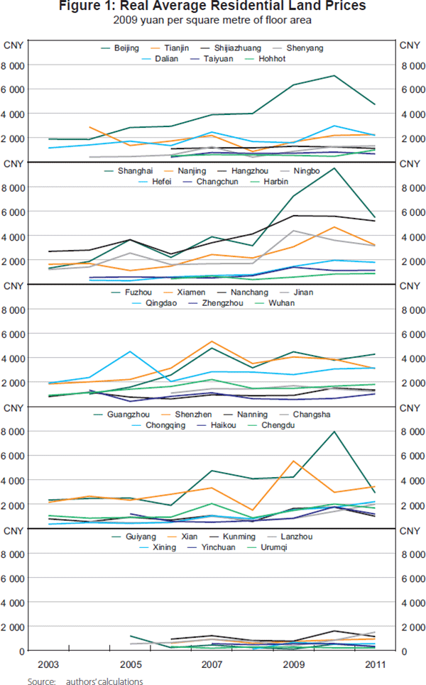
Land parcels in China are priced in terms of the floor area of housing permitted to be built on the parcel, instead of the land area. Real prices in constant 2009 yuan per square metre of permitted space are computed by deflating by the relevant monthly CPI series for each city. Figure 1 plots the simple means of these real values for each year in each market. There is substantial heterogeneity in prices across markets, and one can see the mean reversion that will be documented more formally below. The growing dispersion apparent in Figure 1 is misleading, as it is partially due to the inclusion of additional markets over time. For example, for the 15 markets with complete data throughout our sample period, in 2003 land was nearly eight times more costly in the most expensive market (2693 yuan per square metre of floor area in Hangzhou) than in the least expensive city (352 yuan in Chongqing). By 2011, the gap between the highest and lowest of these 15 markets was just over five times (i.e. with Shanghai at 5,470 yuan and Nanning at 997 yuan per square metre). This is not a small absolute difference by any means, but still pales in comparison to the nearly 25 times gap in 2011 between Shanghai and Urumqi (222 yuan per square metre) for the full sample of 35 markets.
We do not work with the unadjusted transactions prices in the analysis below because they may be driven by quality changes that could arise for a number of reasons. One is that the highest quality sites might be sold first, so that the change in the unadjusted mean values for a given city would understate the true constant quality rate of price appreciation. On the other hand, local governments might reserve the good parcels and only list them during the more recent boom periods of the stimulus years. This would result in an overestimation of price growth in the simple average series. In addition, some land parcels were not levelled on delivery in a few cities in the early years of our sample. Not controlling for this would result in overestimation of true, constant quality price growth.[8] It also is possible that sales of high-quality parcels occur whenever the local government has the greatest need for revenue. Thus, the bias could go in either direction for different markets.
Consequently, we follow Wu et al (2012) in creating constant quality land price indices for each market. Our city-level hedonic price index is estimated using ordinary least squares (OLS), with the log of the real transaction price as the dependent variable. The explanatory variables are: (a) the parcel's distance to the centre of the corresponding city (D_CENTER), which is measured after mapping the precise location of each site with Geographic Information Systems software; (b) the distance to the nearest subway station (D_SUBWAY), which is relevant in 10 of the 35 cities with operating subway systems during our sample period; (c) district dummies which control for local/neighbourhood-level fixed effects not captured by the two previous location controls; (d) a set of physical attributes including the land area of the parcel (SIZE), the density permitted on the site when it was built (FAR) and whether the parcel is levelled on delivery (LEVEL); (e) variables that indicate whether a small portion of the residential land parcel is designated for affiliated commercial properties (COMMERCIAL), public establishments (PUBLIC), or public housing units (PH); (f) the parcel's transaction form as reflected in whether it was purchased via sealed bidding (BIDDING), regular English auction (AUCTION), or two-stage auction (the default group); and (g) year dummies, whose coefficients are used to create the constant quality price index.
Our land price hedonic model works at least tolerably well in each of the 35 cities. The coefficients on the quality controls are generally consistent with expectations, and we always can reject the null hypothesis that they have no explanatory power. Adjusted R2 statistics vary from a low of 0.17 (Urumqi, for which data begin in 2006) to a high of 0.72 (Fuzhou, for which data begin in 2004). Table A1 reports some summary statistics on these underlying regressions, all of which are available upon request.[9] The land price index in each city is constructed from the estimated coefficients of the time dummies, where 2009 is the base year (i.e. year 2009 = 100).[10]
2.2 Land price growth from 2003 to 2011
Implied real, constant-quality compounded average annual growth rates for each of the 35 cities are listed in Table 2. Among the 22 markets with data back at least to 2004, there are only 2 in which constant-quality land price growth is estimated to have appreciated at an average compound rate below 10 per cent (Nanchang and Qingdao, at 7.8 per cent and 5.9 per cent, respectively). Nine have experienced average compound annual growth rates above 20 per cent. Naturally, this implies extremely high aggregate growth in real land values. The greatest price appreciation has occurred in Chongqing, which saw prices escalate by 577 per cent between 2003 and 2011. The analogous figures for Beijing and Shanghai are 336 per cent and 448 per cent.[11] Six of the fifteen markets with data back to 2003 have average compound annual growth rates above 20 per cent, which implies their land prices have grown by more than 330 per cent between 2003 and 2011. Qingdao's relatively low 5.9 per cent per annum average compound growth has led to 2011 prices that are 58 per cent higher than in 2003.
| 15 markets, 2003–2011 8 years |
7 markets, 2004–2011 7 years |
2 markets, 2005–2011 6 years |
9 markets, 2006–2011 5 years |
1 market, 2007–2011 4 years |
1 market, 2008–2011 3 years |
||||||
|---|---|---|---|---|---|---|---|---|---|---|---|
| Chongqing | 27.0 | Hefei | 30.1 | Lanzhou | 20.7 | Hohhot | 19.7 | Yinchuan | 8.9 | Xining | 49.9 |
| Shanghai | 23.7 | Changsha | 20.3 | Guiyang | 12.4 | Haikou | 17.8 | ||||
| Hangzhou | 21.8 | Tianjin | 20.2 | Taiyuan | 12.2 | ||||||
| Nanjing | 20.5 | Fuzhou | 17.7 | Harbin | 10.8 | ||||||
| Beijing | 20.2 | Changchun | 13.9 | Jinan | 7.2 | ||||||
| Shenzhen | 20.1 | Shenyang | 13.7 | Xian | 6.9 | ||||||
| Xiamen | 18.7 | Zhengzhou | 10.3 | Shijiazhuang | 5.1 | ||||||
| Ningbo | 18.5 | Kunming | 2.0 | ||||||||
| Chengdu | 16.7 | Urumqi | −2.9 | ||||||||
| Dalian | 15.8 | ||||||||||
| Guangzhou | 14.7 | ||||||||||
| Wuhan | 13.3 | ||||||||||
| Nanning | 12.3 | ||||||||||
| Nanchang | 7.8 | ||||||||||
| Qingdao | 5.9 | ||||||||||
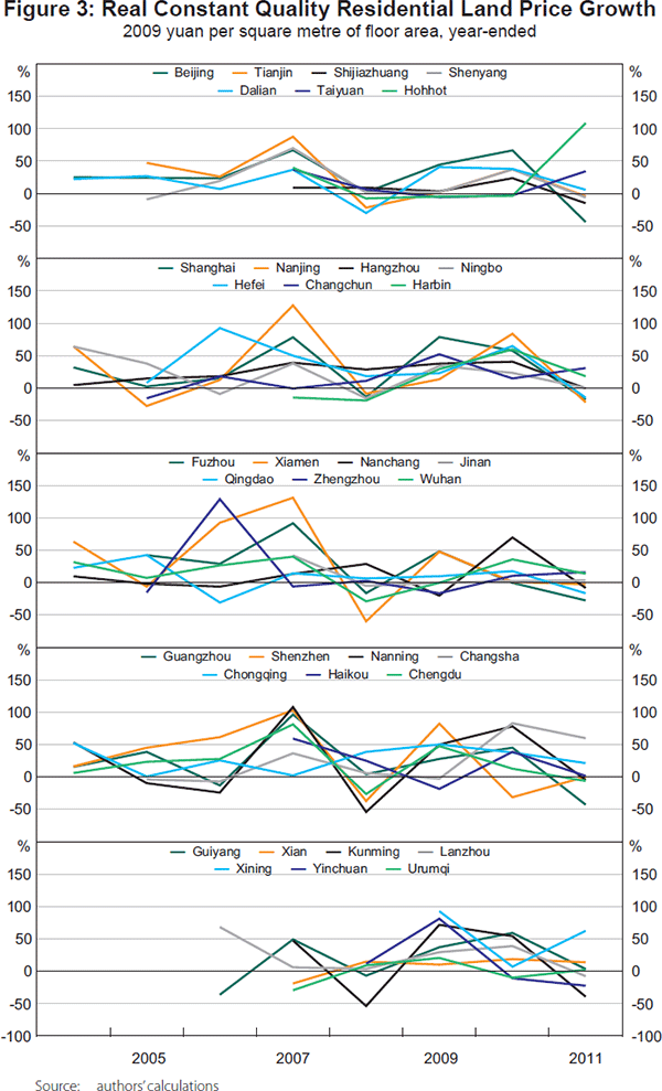
Summary statistics on the distribution of annual appreciation rates over time are presented in Table 3. Double-digit average annual price appreciation is the norm; the simple average across markets is only below 10 per cent in two years and negative only during 2007–2008. The 34 markets with data for that time period were almost evenly split between those experiencing positive and negative price growth. Even though average real land price growth was slightly positive in 2010–2011, more markets saw price declines than increases that period.
| 2003–2004 | 2004–2005 | 2005–2006 | 2006–2007 | |
|---|---|---|---|---|
| Mean – % | 32.1 | 12.2 | 23.5 | 46.4 |
| Standard deviation – % | 21.7 | 23.1 | 40.5 | 42.1 |
| Max – % | 64.1 | 47.2 | 128.8 | 131.2 |
| Min – % | 4.4 | −28.0 | −36.1 | −29.2 |
| Number of cities | 15 | 22 | 24 | 33 |
| Number with positive appreciation | 15 | 15 | 17 | 28 |
| Number with negative appreciation | 0 | 7 | 7 | 5 |
| 2007–2008 | 2008–2009 | 2009–2010 | 2010–2011 | |
| Mean – % | −5.3 | 28.5 | 31.4 | 2.6 |
| Standard deviation – % | 24.0 | 30.7 | 29.4 | 30.2 |
| Max – % | 38.6 | 93.1 | 83.6 | 108.6 |
| Min – % | −59.9 | −20.2 | −31.6 | −44.2 |
| Number of cities | 34 | 35 | 35 | 35 |
| Number with positive appreciation | 18 | 27 | 29 | 16 |
| Number with negative appreciation | 16 | 8 | 6 | 19 |
The extremely high volatility of land prices is also demonstrated in Table 3. There are very wide swings in the mean growth rates across individual years, and there is evidence of mean reversion at annual frequencies. The average absolute difference in mean price growth rates between consecutive time periods is 24.5 per cent. The swing in growth rates upon entering the global financial crisis from 2006–2007 to 2007–2008 was −51.7 percentage points, and the decline from 2009–2010 to 2010–2011 following the end of the stimulus was −28.8 percentage points. The gaps between the markets with the highest and lowest land price growth in any given year also are extremely wide. Those differences range from 60 percentage points in 2003–2004 to 165 percentage points in 2005–2006. While most markets tend to move in the same direction within any one year, individual cities can and do experience outsized booms and busts at given points in time. And, there are generally a handful of local markets in which land prices fall in any given year.
Table 4 provides additional insight into just how volatile land prices have been in Chinese cities. Given that land is the residual claimant on property value in standard models, we would expect it to be more volatile than housing prices overall. The top panel of Table 4 compares simple mean growth rates of housing and land prices over time in our sample of cities, along with similar measures for construction costs and wages in the construction industry.[12] The bottom panel then reports the annual standard deviations of those variables.
| 2004 | 2005 | 2006 | 2007 | 2008 | 2009 | 2010 | 2011 | |
|---|---|---|---|---|---|---|---|---|
| Mean of annual real growth rates | ||||||||
| Housing price | 4.14 | 5.56 | 6.72 | 13.60 | 8.18 | 9.17 | 23.31 | 8.47 |
| Land price | 32.07 | 12.22 | 23.51 | 46.39 | −5.34 | 28.46 | 31.36 | 2.57 |
| Construction cost | 6.26 | 0.12 | 0.22 | 1.26 | 6.77 | −1.87 | 1.76 | na |
| Construction industry wage | 8.24 | 12.38 | 14.19 | 10.73 | 8.56 | 14.62 | 10.26 | na |
| Number of cities included | 15 | 22 | 25 | 33 | 34 | 35 | 35 | 35 |
| Standard deviation of annual real growth rates | ||||||||
| Housing price | 4.91 | 3.64 | 6.13 | 12.41 | 8.31 | 6.39 | 11.60 | 7.82 |
| Land price | 21.68 | 23.06 | 40.52 | 42.11 | 23.98 | 30.72 | 29.44 | 30.22 |
| Construction cost | 2.23 | 1.68 | 1.39 | 1.38 | 2.49 | 1.31 | 1.29 | na |
| Construction industry wage | 5.78 | 4.29 | 4.61 | 5.07 | 4.33 | 9.01 | 4.89 | na |
| Number of cities included | 15 | 22 | 25 | 33 | 34 | 35 | 35 | 35 |
|
Sources: National Bureau of Statistics of China; authors' calculations |
||||||||
Land price growth well exceeds overall housing price growth in all years except 2008 and 2011, when we estimate that land prices either dropped or stagnated, while housing prices increased modestly. In contrast, construction costs were fairly stable over our sample period, with the highest rate of cost growth being 6.8 per cent in 2008. Construction wages grew by more on average in each year, but wage growth still pales compared with land price appreciation. Standard deviations in land price growth range from 22 to 42 per cent, depending upon the year, so the volatility is quite high. These magnitudes are three to four times larger than the standard deviation of any other factor price reported in Table 4.
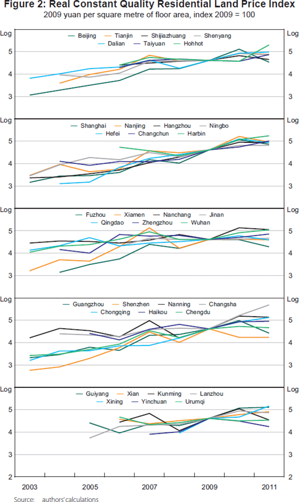
Figure 2 plots the log of each city's land price index, where the price in 2009 is set to 100. Figure 3 plots real land price appreciation rates for the same set of cities. Here, one begins to see the common movement in price growth across markets.
The strong influence of a common, national effect on city-level land price growth is more evident from simple regressions of annual land price appreciation on year and/or city dummies. Table 5 reports summary statistics from these regressions. Year dummies alone can account for 24 per cent of the variation in annual land price growth in the 35 markets depicted in Figure 3. This is more than four times the explanatory power of a regression on the city dummies alone (R2 = 0.05) and one cannot reject the null hypothesis that the city fixed effects are jointly equal to zero. These factors are largely orthogonal to one another, as the explanatory power of the regression that includes them both is R2 = 0.28. Thus, some common, national effect can account for over one-fifth of the variation depicted in Figure 3, while there does not appear to be any fixed city trait that can explain much of it.
| Independent variables | Model | ||
|---|---|---|---|
| (1) | (2) | (3) | |
| Year fixed effect | Yes | No | Yes |
| City fixed effect | No | Yes | Yes |
| R2 | 0.24 | 0.05 | 0.28 |
| Adjusted R2 | 0.21 | −0.11 | 0.13 |
| F-stat for the joint test that all year fixed effects equal 0 | 9.89*** | 8.89*** | |
| F-stat for the joint test that all city fixed effects equal 0 | 0.30 | 0.37 | |
| Number of observations | 233 | 233 | 233 |
| Note: ***, ** and * indicate significance at the 1, 5 and 10 per cent level, respectively | |||
This raises the question of whether there are time-varying local market characteristics which can explain the variation in land price growth. To investigate this, we created a number of variables that reflect demand, supply and credit conditions in each market. The demand for residential land is derived from the demand for housing itself, so one variable to include is a measure of the supply-demand balance in the housing market (hsdratioi,t). More specifically, it is the ratio of the floor area of newly built housing listed in city i and year t (hlistedi,t) to the floor area of newly built housing that was sold in the same city and year (hsoldi,t):

In the regression model estimated below, we introduce the one-year-lagged term, hsdratioi,t − 1, to avoid potential issues associated with reverse causality. This variable should be negatively correlated with the change in local land prices, as a higher value of this ratio indicates increasing oversupply in the housing market.
We also control for expected non-farm employment growth in the city using a variable akin to the one developed by Bartik (1991). This variable, epgrowthi,t, is calculated as the weighted average of national employment growth rates by industry, where the weights reflect each city's share of that industry's aggregate employment. More specifically,

where et is the national employment level in all non-farm industries, ei,j,t is city i's employment in industry j in year t, ẽi,j,t is the national employment level in industry j outside of city i, and the j subscript indexes the 18 non-farm employment sectors in China.[14] This variable should be positively correlated with the change in local land prices, as it is close to being a pure demand shifter.
US credit markets are thought by many to have played a prominent role in helping generate the stark rises in housing prices seen in many US markets. For China, we proxy for local credit market conditions with the amount of new loans issued to developers each year in each market, denominated in billions of 2009 yuan.[15] The specific measure used in the regression analysis below is developloan3yri,t, which is the lagged, three-year average of these loan amounts (i.e. the average for the three years from t – 3 to t – 1). This variable is expected to be positively correlated with changes in local land prices to the extent that easier credit market conditions in the local property market allow developers to bid up land prices.
To see if time-varying local market conditions influence land markets, the log change in the individual city market land price indices is regressed on these factors plus year dummies in a random effects estimation as follows:

where dlogLPi,t is the log change in city i's annual land price index and all other variables are as described above.[16] The results are reported in the first column of Table 6. Note that this table only uses data up to 2010 because that is the latest year available for some regressors.
| Independent variables | Model | |
|---|---|---|
| (1) | (2) | |
| Expected employment growth (epgrowthi,t) |
0.0825 (0.0530) |
0.1722** (0.0696) |
| expgrowthi,t * 2009/10 | −0.2120* (0.1089) |
|
| Previous supply-demand balance in housing (hsdratioi,t−1) |
−0.1245** (0.0603) |
−0.1570* (0.0852) |
| hsdratioi,t−1 * 2009/10 | 0.0231 (0.1222) |
|
| Previous three-year average loan volumes to developers (developloan3yri,t) |
0.0019* (0.0011) |
0.0013 (0.0017) |
| developloan3yri,t * 2009/10 | 0.0011 (0.0023) |
|
| Year fixed effect | Yes | Yes |
| City fixed effect | No | No |
| R2 | 0.27 | 0.29 |
| Number of observations | 183 | 183 |
| Notes: Standard errors in parentheses; ***, ** and * indicate significance at the 1, 5 and 10 per cent level, respectively; 16 observations are dropped due to the missing value in hsdratioi,t – 1 | ||
Each coefficient has the expected sign, with those on the supply-demand conditions and liquidity measures being statistically significant at standard confidence levels. The expected employment growth variable is significant at the 12 per cent level. The second column of Table 6 augments this baseline specification by including interactions of each local trait with a dummy variable indicating the period after the global financial crisis began and China instituted its massive stimulus program (i.e. 2009 and 2010). Here, we see that virtually all of the impact of the time-varying local traits is due to variation in the years prior to 2009. While caution is in order given the limited degrees of freedom involved, we cannot find any local trait that is strongly correlated with land price changes in a statistical or economic sense during the stimulus period.
Even prior to the stimulus, the economic importance of these traits is limited. Computing standardised marginal effects of the three local characteristics using the coefficients from column (2) of Table 6 yields the following: (a) a one standard deviation increase in expected employment growth in a city is associated with an increase in the log change of its land prices of one-fifth of a standard deviation; (b) a one standard deviation increase in the ratio of floor space listed relative to that sold in the market in the previous year is associated with the log change of local land prices falling by half of a standard deviation; and (c) a one standard deviation increase in the lagged average of developer loans in the city is associated with an increase in the log change in land prices of about one-tenth of a standard deviation.
In one sense, it is comforting to know that our proxies for local market fundamentals and credit conditions work as any simple economic model would predict, especially given the limited time series over which we can estimate the relationships.[17] However, it still is the case that these effects are small relative to the impact of the common national effects reflected in the coefficients on the year dummies. On average, the typical ‘year effect’ explains about 30 per cent, which is roughly equal to one standard deviation of the log change in annual land prices for the cities in our sample. This suggests that changes in sentiment about the country's economic prospects will influence local land markets more than the supply-demand fundamentals of those markets themselves.
One other noteworthy feature of Figure 3 is the mean reversion apparent in the series. Table 7 reports results from very simple models of the log change in current land price appreciation on its lag, controlling for time and city fixed effects (in most cases). One does not want to make too much of these findings given the limited time series (and the fact that we do not have data over a complete housing cycle), but the findings confirm the visual impression delivered by Figure 3. Essentially, if land price growth is 1 percentage point higher this period, it is about 0.35 per cent lower next period (column (1)). This is quite different from what researchers have found in the housing market in US where there is strong persistence in housing price growth across years and mean reversion over longer periods such as five-year intervals (e.g. Case and Shiller (1987), Cutler, Poterba and Summers (1991), Glaeser et al (2010)).
| Independent variables | Model | |||
|---|---|---|---|---|
| (1) | (2) | (3) | (4) | |
| dlog(LPi,t−1) | −0.3527 (0.0764)*** |
−0.4427 (0.0891)*** |
−0.4243 (0.0749)*** |
−0.5961 (0.0864)*** |
| dlog(LPi,t−2) | −0.1905 (0.0888)** |
−0.3806 (0.0868)*** |
||
| YEAR2006 | −0.0156 (0.0909) |
|||
| YEAR2007 | 0.2479 (0.0891)*** |
0.3149 (0.0875)*** |
||
| YEAR2008 | −0.1850 (0.0857)** |
−0.1175 (0.0885) |
||
| YEAR2009 | −0.0273 (0.0887) |
0.0302 (0.0840) |
||
| YEAR2010 | 0.1151 (0.0849) |
0.1459 (0.0865)* |
||
| YEAR2011 | −0.1354 (0.0849) |
−0.0567 (0.0832) |
||
| Constant | 0.2114 (0.0732)** |
0.1978 (0.0734)*** |
0.2131 (0.0249)*** |
0.3038 (0.0330)*** |
| City fixed effect | Yes | Yes | Yes | Yes |
| R2 | 0.34 | 0.36 | 0.12 | 0.17 |
| Number of observations | 198 | 163 | 198 | 163 |
| Notes: Standard errors in parantheses; ***, ** and * indicate significance at the 1, 5 and 10 per cent level, respectively | ||||
This naturally raises the question of why this pattern exists in the data, and whether the volatility in the land prices provides useful information to understand housing price movements. We do not answer that question here, but Table 8 provides some intriguing insight into one possible factor. The Chinese Government is known to intervene in the housing market, especially to tame it. For instance, when housing markets in some coastal region cities started to boom in 2004–2005, the central government issued a series of intervention policies between late 2005 and early 2006 to cool the market. Similar patterns also apply to the cases of intense interventions in late 2007, where the effect was later intertwined with the global financial crisis, and more recently in the second half of 2010. The huge stimulus package in December 2008, and the introduction of measures focusing on encouraging housing consumption around the same time (State Council Decree, No [2008]131), are a counter-example because they may have at least partially fuelled the skyrocketing housing prices and land prices in 2009. The results in Table 8 lend credence to a role for the government. The first specification interacts the lagged land price appreciation term with a dummy variable indicating the direction of land price growth in the previous year. The results indicate that mean reversion is larger if land prices were increasing in the previous year. Subsequent specifications in Table 8 investigate whether local fiscal conditions might also have played a role. Those specifications include a triple interaction variable deficiti,t, (that includes the size of the local fiscal deficit in the previous year), which is calculated as the ratio between local budgetary fiscal expenditure bexpi,t and budgetary income binci,t in city i and year t,

| Independent variables | Model | |||
|---|---|---|---|---|
| (1) | (2) | (3) | (4) | |
| dlog(LPi,t−1) * (dlog(LPi,t−1) ≥ 0) |
−0.4323 (0.1173)*** |
−1.1490 (0.5071)** |
−0.5528 (0.1203)*** |
−1.6853 (0.5165)*** |
| dlog(LPi,t−1) * (dlog(LPi,t−1) ≥ 0) * deficiti,t−1 |
0.4626 (0.3674) |
0.8139 (0.3860)** |
||
| dlog(LPi,t−1) * (dlog(LPi,t−1) < 0) |
−0.2039 (0.1831) |
0.3254 (0.8092) |
−0.1770 (0.1963) |
0.7549 (0.8846) |
| dlog(LPi,t−1) * (dlog(LPi,t−1) < 0) * deficiti,t−1 |
−0.3903 (0.5952) |
−0.6748 (0.6557) |
||
| Constant | 0.2290 (0.0759)*** |
0.2177 (0.0777)*** |
0.2542 (0.0391)*** |
0.2888 (0.0424)*** |
| Year fixed effect | Yes | Yes | Yes | Yes |
| City fixed effect | Yes | Yes | Yes | Yes |
| R2 | 0.34 | 0.29 | 0.13 | 0.09 |
| Number of observations | 198 | 163 | 198 | 163 |
| Notes: Standard errors in parantheses; ***, ** and * indicate significance at the 1, 5 and 10 per cent level, respectively | ||||
In the analysis, deficiti,t serves as the proxy of a local government's fiscal pressures and reliance on land sales.[18] The coefficients on this term are not statistically significant at standard confidence levels, but the sign indicates that mean reversion from price growth booms is smaller if the local government has been running larger deficits. Perhaps governments running larger deficits have less of an incentive to actively implement any countervailing policies emanating from the central government in Beijing. In contrast, when price growth has been falling, such cities might have an incentive to be especially aggressive in reversing the decline in prices, which would lead to the larger mean reversion effect. The pattern of these results is consistent with this expectation, although it is at most marginally significant. We certainly have not established any causal relationships, but the exercise does serve to illustrate the potential usefulness of a rich panel of observations on local land markets.
2.3 Stylised facts about quantities: the volume of land sales during 2003–2010
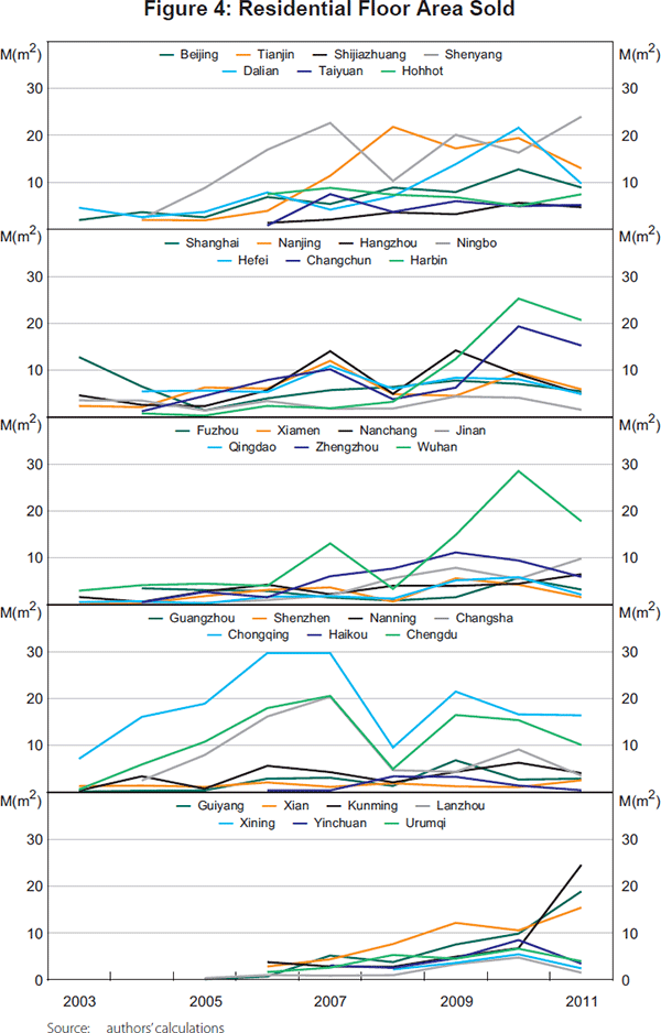
Figure 4 plots the floor area sold by year across our sample of markets. Table 9 reports summary statistics on the amount of space supplied. Note that the supply of space has increased greatly, and this is not solely due to the rise in the number of cities covered in our sample. The aggregate supply of space has roughly doubled just since 2008, when all 35 cities are included in the sample. Figure 4 also depicts some convergence in the flow amount of new space supplied across markets over time.[19]
| Mean | Standard deviation | 25th percentile | Median | 75th percentile | Number of cities included | |
|---|---|---|---|---|---|---|
| 2003 | 2.86 | 3.13 | 0.53 | 1.89 | 4.52 | 15 |
| 2004 | 3.25 | 3.43 | 1.16 | 2.52 | 3.58 | 22 |
| 2005 | 3.98 | 4.31 | 1.32 | 2.59 | 5.55 | 24 |
| 2006 | 5.62 | 6.25 | 1.68 | 3.79 | 6.02 | 33 |
| 2007 | 7.46 | 7.17 | 2.11 | 4.33 | 11.35 | 34 |
| 2008 | 5.34 | 4.29 | 2.52 | 4.41 | 7.48 | 35 |
| 2009 | 8.04 | 5.72 | 4.55 | 6.20 | 12.36 | 35 |
| 2010 | 10.13 | 6.94 | 5.21 | 7.36 | 13.45 | 35 |
| 2011 | 9.26 | 7.84 | 3.20 | 6.33 | 12.96 | 35 |
Table 10 reports results analogous to those in Table 5, demonstrating whether this movement in supply can be explained by city or time fixed effects. Both factors are empirically relevant, although city fixed effects can explain more of the variation. It is not surprising to find significant city fixed effects here, as the amount of space supplied is certainly linked with market scale. However, there are statistically and economically meaningful year effects, so we cannot reject the null hypothesis of a strong common or national effect in new supply.
| Independent variables | Model | ||
|---|---|---|---|
| (1) | (2) | (3) | |
| Year fixed effect | Yes | No | Yes |
| City fixed effect | No | Yes | Yes |
| R2 | 0.22 | 0.42 | 0.68 |
| Adjusted R2 | 0.20 | 0.34 | 0.60 |
| F-stat for the joint test of all year fixed effects equalling 0 | 8.34*** | 18.18*** | |
| F-stat for the joint test of all city fixed effects equalling 0 | 5.03*** | 8.87*** | |
| Number of observations | 268 | 268 | 268 |
| Note: ***, ** and * indicate significance at the 1, 5 and 10 per cent level, respectively | |||
Table 11 reports some simple regressions to see if time-varying city traits can explain any of the variance in the supply series. Here, besides the city and year fixed effects, we introduce two local politics variables. One measures the degree of budgetary deficit in the previous year as defined above, and the other measures the length of time (in years) that the top local Chinese Communist Party (CCP) officer has been in his (or her) position. The results in column (1) of Table 11 show that if the city government was spending a lot relative to its revenues in the previous year, it is likely to sell more land this year. In addition, the more land that gets supplied the newer is the top CCP officer in the local government.[20] While these results should be viewed as simple correlations they strongly suggest that local political economy considerations play an economically meaningful role in land supply developments. The second column of Table 11 includes interaction terms with the stimulus period of 2009–2010. Both coefficients are positive, but neither is statistically significant. Columns (3) and (4) investigate whether current deficit situations (not just lagged ones) are correlated with supply conditions (this variable is only available until 2010). The answer is yes, and the finding that CCP officers new to their offices sell more land is robust to these changes in specification.
| Independent variables | Model | |||
|---|---|---|---|---|
| (1) | (2) | (3) | (4) | |
| Degree of budgetary deficit in the previous year (deficiti,t−1) |
0.9488** (0.4253) |
0.7862* (0.4573) |
||
| deficiti,t−1 * 2009/10 | 0.3012 (0.3084) |
|||
| Degree of budgetary deficit in the current year (deficiti,t) |
1.1884*** (0.4407) |
1.0838** (0.4840) |
||
| deficiti,t * 2009/10 | 0.1372 (0.2931) |
|||
| Length of CCP top officer in current position (lengthi,t) |
−0.0558* (0.0285) |
−0.0713** (0.0344) |
−0.0569** (0.0283) |
−0.0674* (0.0344) |
| lengthi,t * 2009/10 | 0.0406 (0.0523) |
0.0273 (0.0522) |
||
| Year fixed effect | Yes | Yes | Yes | Yes |
| City fixed effect | Yes | Yes | Yes | Yes |
| R2 | 0.22 | 0.21 | 0.19 | 0.19 |
| Number of observations | 234 | 234 | 234 | 234 |
| Notes: Standard errors in parantheses; ***, ** and * indicate significance at the 1, 5 and 10 per cent level, respectively | ||||
In sum, city and year fixed effects can explain about 60 per cent of the variation in the supply of new space annually in our 35 market sample. Local political economy factors also appear to be empirically relevant, as the fiscal balance of the city and whether the local CCP chief is new to his or her job also are correlated with supply.
2.4 Some final comments on very recent changes in Chinese land market data
The widespread, but not universal, declines in real constant quality land prices in 2011 are similar in nature to what happened in 2008 as the global financial crisis unfolded. Nineteen markets saw real land values fall in 2011 versus sixteen in 2008. Those earlier period declines were quickly reversed by the massive Chinese Government stimulus in 2009 and 2010. Only time will tell if something similar occurs this time.
There is still substantial heterogeneity across markets, even in the most recent data, so it remains inaccurate to claim that there is some single national Chinese land or property market. Sixteen markets still experienced positive land price growth in 2011, and nine of them had double-digit price growth (and each of these nine were in the interior of the country).[21] There were some very big price declines too, with ten of the nineteen cases of falling prices experiencing double-digit drops. Many of these markets were along or near China's coast.[22]
We have also collected data for the first quarter of 2012. These city-level samples are small, so we do not report price index or change data. However, there are stark falls in transaction volumes, whether measured by the number of parcels sold or by the permitted square metres on those parcels. Using the latter metric, 2012:Q1 volumes are 65 per cent of their 2011:Q1 levels and 46 per cent of 2010:Q1 levels, on average. In only 6 of our 35 markets are permitted square metres on sold parcels in the first quarter of 2012 greater than that in the first quarter of 2011; the analogous number when comparing 2012:Q1 to 2010:Q1 is seven.[23] In 21 of the 35 markets (or 60 per cent of our sample), levels of permitted square metres in 2012:Q1 that are at least 50 per cent below levels prevailing in 2010:Q1. The changes here are especially stark among the coastal markets: Beijing's numbers are down by 75 per cent; Shanghai's by 91 per cent; Fuzhou's by 96 per cent; Dalian's by 92 per cent; Qingdao's by 91 per cent; Ningbo's by 89 per cent; Guangzhou and Xiamen had no land sales in 2012:Q1, so their levels are down by 100 per cent. These percentage changes are not artificially high because of the comparison with the 2010:Q1 stimulus period. Twenty-two of our thirty-five markets have permitted square metres on sold land parcels in the first quarter of 2012 that are more than 50 per cent below their levels in the first quarter of 2011.
In sum, transaction volumes in the land market have plummeted in most (but not all) major Chinese cities in the first quarter of 2012. This suggests that demand from private developers is very low. It is well known that house prices around the world do not follow a random walk (e.g. Case and Shiller (1989)) and tend to be sticky downward with quantities falling before prices do. If this is the case in China, then these most recent transaction data are foreboding and bear close scrutiny going forward. If they do not reverse to a significant extent, one would expect sharp price declines in the near future.
3. What is the True Level of Housing Price Growth in China? Measurement and Analysis
Measuring housing price growth may seem like a straightforward matter given the now-widespread acceptance of the repeat-sales methodology reintroduced and popularised by Case and Shiller (1987, 1989).[24] However, it is not so in China (and other emerging markets), where a significant portion of the housing stock consists of new (or relatively new) housing units that have not yet been sold multiple times. Obviously, a repeat-sales index captures price changes of existing homes, which by definition are the only ones that have been sold more than once.
China reports two housing price series, each of which is based exclusively on the values of newly built housing units. According to statistics published by MHURD, 64 per cent of all the floor space transacted in 2010 was from newly built units, so accurately measuring the price change on new units captures much of the variation in the value of entire housing stock in China.[25]
One series is the called the ‘Average Selling Price of Newly Built Residential Index’. This is the simple average of transaction prices (total sales value divided by total size of housing unit transacted) on new housing units, and is based on statistics reported by all developers in each market. It makes no attempt to control for any quality differential across markets or drift in the quality (positive or negative) in housing units over time. It is available for all markets across China. The other series, which is officially termed ‘Price Indices in 70 Large and Medium-Sized Cities’ (‘70 cities index’), is a measure of changes in average prices on unit sales within individual housing complexes over sales stage or time. More specifically, this index is calculated by first computing the average sale price of new units each month, by housing complex. The monthly series is then the average of each complex's average price changes over time weighted by transaction volume.
Figure 5 plots each series for the eight major markets reported in Wu et al (2012) between 2006:Q1 and 2010:Q4.[26] Table 12 reports the implied average compound price growth for each series over our sample period. There are two noteworthy features of these data. First, data from the ‘70 cities index’ never show much price appreciation in any of the eight major markets. In some, but not all, of these cities, the simple average price index also exhibits relatively little growth and volatility. Second, the two series are not highly correlated with one another.
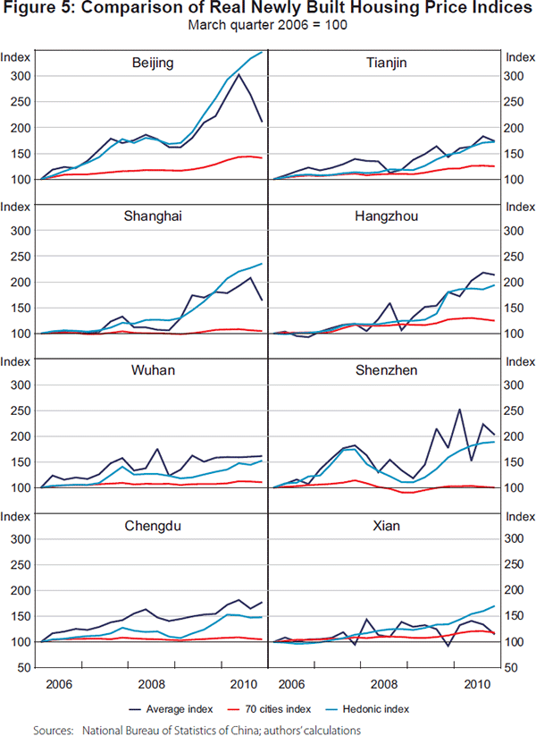
| City | Average index | 70 cities index | Hedonic index |
|---|---|---|---|
| Beijing | 4.00 | 1.83 | 6.77 |
| Tianjin | 2.95 | 1.18 | 2.90 |
| Shanghai | 2.63 | 0.25 | 4.61 |
| Hangzhou | 4.08 | 1.17 | 3.54 |
| Wuhan | 2.56 | 0.54 | 2.25 |
| Shenzhen | 3.78 | 0.01 | 3.40 |
| Chengdu | 3.06 | 0.27 | 2.08 |
| Xian | 0.73 | 0.89 | 2.84 |
|
Sources: National Bureau of Statistics of China; authors' calculations |
|||
If these data are to be believed, the ‘70 cities index’ in particular sends a comforting message about the state of housing markets in major Chinese cities, in that they do not indicate there has been a boom that might have led to substantial overpricing (relative to underlying fundamentals) of housing prices in these places. However, Wu et al (forthcoming) provide good reasons to believe these series are biased downward, possibly quite substantially. For example, it is well known that price growth calculations based on simple averages will overstate (understate) the true change in constant quality values to the extent that quality rises (falls) over time. To determine the extent of heterogeneity across markets and quality drift over time, one must go to the data.
The continuous suburbanisation of sites as urban growth has skyrocketed in major Chinese cities means that new units are being produced in housing complexes farther away from the urban core. Using data on an anonymous Chinese market, Wu et al (forthcoming) report that the average distance from the city centre increased by 50 per cent between 2004 and 2007 (i.e. from 4.2 kilometres to 6.1 kilometres). If this is typical of most rapidly growing markets, then location quality has changed a lot in recent years. In the US context, this would not be a signal of lower quality, as sorting into suburban sites is often associated with higher location quality, particularly as higher-income households sort into homes located in high-quality school districts. There is no reason to expect any such spatial sorting in China, and Wu et al (forthcoming) report results from a hedonic housing price regression (see below for more on their model and the hedonic approach) indicating that not controlling for the fact that new housing units are being built farther out from the urban core is associated with more than a 14 per cent underestimation of constant quality prices. Hence, the rapid growth in urban Chinese markets is associated with units being built on lower-quality sites, and not controlling for this feature results in a meaningful underestimation of constant quality price growth over a period as short as three years.[27]
Increasing density is another trait of new housing complexes that suggests quality has deteriorated over time. Based on data from various issues of the Statistics Yearbook of China, Wu et al (forthcoming) calculate that permitted floor area ratios (FAR) increased by over 60 per cent between 2000 and 2010 (i.e. from 2.15 in 2000 to 3.57 in 2010). Their hedonic analysis, using micro data on an unnamed Chinese housing market, indicates this does not severely depress prices, but increasing density is considered a disamenity in any reasonable housing or urban model, so it is yet another reason why the two government indices might understate true price growth, all else constant.[28]
Strategic pricing behaviour by developers is yet another reason why the second ‘70 cities index’ might substantially understate true housing price appreciation. As Wu et al (forthcoming) argue, the trade-off between setting a higher price and the carry costs of unsold units, as reflected in their time on the market, is likely to lead developers to price their units so the last units sold are of lower price. In their empirical analysis using data from the same anonymous Chinese housing market, they provide results from a hedonic regression that is consistent with this conclusion, as the last unit sold in a typical housing complex goes for 11 per cent less than the first unit sold in the same complex. Thus, not being able to control for the timing of sales, which the ‘70 cities index’ does not do, is likely to lead to substantial underestimation of the true price increase.
Even if individual housing unit quality has not deteriorated over time (and it could have increased), all this suggests that the quality of the housing complexes in which the units are located has fallen over time, probably because of their inferior locations.[29] Not being able to control for this downward quality drift means that both indices reported by the government underestimate the true extent of housing price growth.[30]
Therefore, we apply the hedonic estimation approach to all the newly built housing units transacted between 2006 and 2010 in the eight major cities reported by Wu et al (2012).[31] The resulting series and their real average compound growth rates are reported in Figure 5 and Table 12. There are two noteworthy features of the comparison between this constant quality index and the two existing official indices. First, in each of the eight cities the hedonic indices grow much faster than the ‘70 cities index’. The deviation from the real average compound price growth rates varies from 1.7 percentage points in Wuhan to 4.9 percentage points in Beijing. This implies that the bias arising from the strategic pricing behaviour by developers in the newly built markets is important. The ‘70 cities index’, which is presently the most influential housing price indicator in China, appears to be fairly unreliable in terms of capturing price changes over time.[32]
The relationship between the hedonic price index and the average price index is mixed. The average compound growth rate of the hedonic price index is higher in the cities of Beijing, Shanghai and Xian, but fairly similar in Tianjin, Hangzhou, Wuhan and Shenzhen. In Chengdu, the average price index grew faster than the hedonic price index during the sample period. As suggested above, the key potential bias facing the simple average method is due to quality shifts of transacted units, which would vary with time and by city. In general, the eight cities covered here are the most developed cities in China, in which the process of urban expansion started earlier and has slowed in recent years. This suggests that the effect of urban expansion on the average price index would be more important in the emerging cites. Even though it seems that the bias in the average price index in these eight major markets would not significantly affect our judgment of their market conditions during the sample period, we still would not want to extrapolate that conclusion to other markets or to the national level.[33]
Another difference is that the average price series is always more volatile than the hedonic price index, which at least partially reflects fluctuation in the quality of units sold. This effect is especially important in relatively small markets such as Shenzhen and Xian, and will make the change in the average price index in specific periods less reliable, such as the sharp fluctuation of the average price index in Shenzhen in 2009 and 2010. Even in large markets like Beijing and Shanghai, such an effect could lead to very different results in some periods like late 2010.
4. Summary and Conclusion
This paper reports the first results and summary statistics on conditions in Chinese land markets using new data based on auction sales from 2003–2010 in 35 major cities. While there is meaningful heterogeneity in land price growth across markets, on average, the nine years to 2011 saw land values skyrocket in many markets, not just those on the coast. The typical market has experienced double-digit compound annual growth in real values on average.
Three notable characteristics about the land price growth series are their strong mean reversion at annual frequencies, the strong common factor in their movements, and their very high volatility. Mean reversion is about 35 per cent from one year to the next. Year dummies account for just over one-fifth of the variation in these data, while city fixed effects are not statistically significant. Volatility is quite high in comparison with other factors of production used in housing, suggesting that the volatility in housing prices is being driven by the land market, not construction costs or construction sector wages.
Quantities, not just prices, have been increasing sharply in recent years. The amount of space supplied has typically doubled since 2008. The supply of land is better explained by city-specific factors, although there is some common, year effect, too. Local political economy factors can account for some of the variation in supply over time within cities.
We also investigated the quality of the two most prominent housing price indices in China, and concluded that a traditional hedonic price index would more accurately reflect how housing prices have changed over time in eight major markets in China. Repeat-sales indices have become standard in many markets, but they are not as useful in emerging markets, such as China, because the bulk of the housing stock is relatively new and has not traded multiple times. China's most prominent index, which reflects changes in the averages of sales within a housing complex over time, shows very little volatility and limited overall price appreciation. It appears to suffer from severe downward bias for the reasons discussed in Wu et al (forthcoming). A simpler average price index, also published in China, shows marked rises in some markets, but not in others. It appears to be most biased downward where quality change has been the greatest. This tends to be in the smaller and emerging markets. We conclude that simple hedonic price indices that can control for basic unit traits, as well as the quality of the housing complex's location, capture changes in housing prices over time more accurately in most markets. Hedonic price indices show very high housing price appreciation over time and appear to reflect the path of housing prices in Chinese markets more accurately.
We believe these data will serve as the foundation for much broader and in-depth future work on Chinese land and housing markets. There is much more to be done in investigating how local market traits might explain the time series variation documented here more effectively. Other potentially important questions include whether changes in local land prices are good predictors of what will happen to housing prices in the future and whether there is an economically important collateral channel effect for non-real estate sector firms seeking credit through the Chinese finance system.
Appendix A
| City | Starting year | Number of observations | Adjusted R2 |
|---|---|---|---|
| Beijing | 2003 | 355 | 0.640 |
| Tianjin | 2004 | 369 | 0.459 |
| Shijiazhuang | 2006 | 94 | 0.425 |
| Taiyuan | 2006 | 141 | 0.360 |
| Hohhot | 2006 | 276 | 0.325 |
| Shenyang | 2004 | 654 | 0.494 |
| Dalian | 2003 | 473 | 0.620 |
| Changchun | 2004 | 373 | 0.350 |
| Harbin | 2006 | 354 | 0.525 |
| Shanghai | 2003 | 460 | 0.653 |
| Nanjing | 2003 | 367 | 0.592 |
| Hangzhou | 2003 | 565 | 0.663 |
| Ningbo | 2003 | 239 | 0.491 |
| Hefei | 2004 | 336 | 0.561 |
| Fuzhou | 2004 | 153 | 0.723 |
| Xiamen | 2003 | 150 | 0.715 |
| Nanchang | 2003 | 251 | 0.379 |
| Jinan | 2006 | 232 | 0.367 |
| Qingdao | 2003 | 161 | 0.444 |
| Zhengzhou | 2004 | 214 | 0.242 |
| Wuhan | 2003 | 486 | 0.418 |
| Changsha | 2004 | 495 | 0.294 |
| Guangzhou | 2003 | 139 | 0.380 |
| Shenzhen | 2003 | 66 | 0.455 |
| Nanning | 2003 | 218 | 0.237 |
| Haikou | 2006 | 61 | 0.184 |
| Chongqing | 2003 | 906 | 0.584 |
| Chengdu | 2003 | 553 | 0.694 |
| Guiyang | 2005 | 162 | 0.177 |
| Kunming | 2006 | 175 | 0.251 |
| Xian | 2006 | 357 | 0.437 |
| Lanzhou | 2005 | 76 | 0.485 |
| Xining | 2008 | 93 | 0.240 |
| Yinchuan | 2007 | 97 | 0.348 |
| Urumqi | 2006 | 317 | 0.171 |
Footnotes
The authors acknowledge the sponsorship from the Representative Office for Asia and the Pacific of the Bank for International Settlements (BIS) under the initiative on ‘Property Markets and Financial Stability’. We also thank the participants at the BIS Basel and BIS Hong Kong seminars for their valuable comments. Gyourko thanks the Global Research Initiatives Project of the Wharton School at the University of Pennsylvania for financial support. Deng and Wu thank the Institute of Real Estate Studies at the National University of Singapore for financial support. Wu also thanks the National Natural Science Foundation of China for financial support (No 71003060). We gratefully acknowledge Jia He and Mingying Xu for excellent research assistance. [*]
For some recent examples, see Anderlini (2011), Chovanec (2011) and Krugman (2011). [1]
Technically, Xining has a higher annual rate of appreciation of 49.9 per cent, but we only have three years of data on that market. [2]
One important factor appears to be inferior location or site quality, as rapid urbanisation pushes new buildings further out along the urban periphery of many Chinese cities. The underlying hedonic traits controlled for in our estimation are described below in more detail. [3]
In the US context, Haughwout, Orr and Bedoll (2008) is one counter-example. See Ching and Fu (2003) and Ooi, Sirmans and Turnbull (2006) for a discussion of land transactions observed in Hong Kong SAR and Singapore, respectively. [4]
Prior to this ruling, called the 11th Provision, most transactions of urban land parcels were done by negotiation between a developer and a local government. This process was criticised for being opaque and open to corruption. For our purposes, the prices that resulted seem likely to be below free market levels, with the degree unknown and possibly changing over time depending upon local circumstances. Currently, all transactions must be done via public auctions, including regular English auctions (pai mai), two-stage auctions (gua pai), and sealed biddings (zhao biao). See Cai, Henderson and Zhang (2009) for a comparison of these three types of auctions. [5]
Our data exclude parcels wholly designated for public housing units because the pricing mechanism for those sites is different. Public housing programs in China include low-rent units (lian zu fang), public rental units (gong gong zu lin fang), affordable housing units (jing ji shi yong fang) and price-controlled units (xian jia fang). Typically the parcels designated for low-rent units would be directly allocated by local governments, while parcels for price-controlled units are required to transact via public auctions. [6]
We actually observe the specific date of the land sales, but have limited sample sizes at monthly and quarterly frequencies. Hence, our analysis does not investigate higher frequency periods. [7]
If a land parcel is not levelled on delivery, the purchaser has to pay additional cost for relocating previous occupiers of the parcel, removing the existing buildings, and so forth, which would negatively affect the transaction price of the parcel. Before 2003, whether a parcel was levelled upon delivery was a key part of the negotiation between the developer and the local government. After that, most land parcels sold via public auctions are levelled on delivery, although there were a few exceptions in some cities, especially during the early years. We directly control for this in the hedonic estimation as described below. [8]
We also conducted a two-stage Heckman estimation to control for potential bias arising from the fact that there were a total of 614 parcels listed that failed to result in transactions (either because there were no bidders if there was an auction or the bid prices were lower than the local government's reserve price, which is relevant for cases involving sealed bids). If these failures are disproportionately concentrated in certain periods such as the financial crisis, selection bias would result in an overestimation of the price index for that period. We could not find any statistically significant indications of sample selection bias based on the inverse Mills ratio estimated from the first-stage probit model. [9]
Average annual appreciation in our hedonic price index is about 5 percentage points higher than in the unadjusted price series, which suggests that parcel quality has been falling over time on average. This does vary by time and market to some extent. [10]
Hefei's real land values grew 531 per cent between 2004 and 2011. [11]
The housing price growth rate is derived from the constant quality price index for newly built housing units, which will be described in detail in Section 3. Construction costs and wages in the construction industry are both reported by the National Bureau of Statistics of China (NBSC); since no city-level statistics are available for these two series, the series in the corresponding provinces in which the cities are located are adopted instead. All four series in Table 4 are in real terms and are deflated by the CPI index in each city. Construction cost and wage data for 2011 are not yet available. [12]
The numerator and denominator are based on data provided by the Ministry of Housing and Urban-Rural Development (MHURD). Each reflects activity permitted by a local housing authority. This variable is only available until 2010. [13]
All employment data are from the NBSC. Because industrial classifications were adjusted in 2003, this variable is available in a consistent format beginning in 2004. Currently the data are only available until 2010. [14]
These data are sourced from the NBSC. [15]
We also experimented with directly controlling for city fixed effects. The standard Hausman test indicates the random effects specification is preferred; however, the results are robust to using city fixed effects. [16]
We experimented with other local traits, but they were insignificant and/or did not change the basic tenor of the results reported in Table 6. For example, we also collected data on local infrastructure investments related to transportation, environmental projects (e.g. drainage, purification, gardening and greening), and so-called basic infrastructure (e.g. water supply) as reported by MHURD. Those measures are highly positively correlated with our developer loan variable (the correlation ranges from 0.77 to 0.86 depending upon the specific infrastructure measure). Including one of these infrastructure variables in lieu of our credit market proxy yields very similar results to those reported in Table 6. We also developed a measure of expected time on the market using data on local housing inventory and the amount of sales. This variable is positively correlated with our supply-demand ratio hsdratio, and has no independent influence. However, it is correlated with log land price changes in the expected way. This highlights that our goal here is not to claim some type of tight causal relationship for a specific variable; we have too short a time frame and lack plausibly exogenous variation for such a convincing analysis. Rather, our point is to note that there are various local traits that plausibly capture fundamental conditions which are correlated with land price appreciation in ways that a simple economic model would predict. [17]
In China, local governments' fiscal income mainly comes from two sources: budgetary income from local tax, and off-budget income, most of which is from land sales. Under the current ‘tax revenue sharing system’ established in 1994, local governments can only retain 40–50 per cent of the budgetary income, but are burdened with 70–80 per cent of the budgetary expenditure, which places heavy fiscal pressure on them. Consequently, local governments have to rely on land sales as a major off-budget income source. According to a report by the Ministry of Finance of China to the National People's Congress, in 2010, total land sales income reached 2 914.7 billion yuan nationally, equaling 74.1 per cent of local governments' budgetary income. See Tsui (2005) for more details about the current public finance system in China. [18]
There is a similar convergence if we restrict the sample to the 15 markets for which we have consistent data back to 2003. [19]
Other research suggests that performance in boosting local economic growth is a key determinant of local officers' career path in China (Li and Zhou 2005). The newly appointed officers are strongly incentivised to expand government expenditure or investment more aggressively to build political capital for their future promotions, and thus generate higher demand for fiscal revenues. [20]
Those markets are Changchun (30.8 per cent), Changsha (59.8 per cent), Chongqing (21.2 per cent), Harbin (18.1 per cent), Hohhot (108.6 per cent), Wuhan (13.6 per cent), Xian (14.0 per cent), Xining (62.4 per cent), and Zhengzhou (16.1 per cent). [21]
The biggest declines were in Beijing (−44.2 per cent), Fuzhou (−27.7 per cent), Guangzhou (−43.0 per cent), Shanghai (−18.0 per cent), and Qingdao (−16.6 per cent). The other coastal markets of Dalian, Ningbo, Hangzhou, Shenzhen and Xiamen were either flat or slightly negative. [22]
Only Changsha, Changchun, Chengdu, Jinan, Wuhan, Yinchuan and Zhengzhou have levels of permitted square metres above those during the stimulus period in the first quarter of 2010. [23]
Their work is based on the seminal contribution of Bailey, Muth and Nourse (1963). [24]
Ideally, one would like to capture price changes on existing housing, too, but currently the reported transaction prices of existing units are not considered to be of high quality in China, at least partially because an unknown number of people are reporting lower values to avoid transaction taxes and capital gain taxes. [25]
The average price index started in the mid 1990s, and the ‘70 cities index’ started in 1997. Both indices significantly adjusted the coverage or estimation method in the second half of 2005, and hence here we only display each series since the first quarter of 2006. [26]
That said, accurately controlling for this trait is difficult in a period of extremely high growth. If the true centre of activity is changing, we would expect an unchanging noisy measure to lead to a downwardly biased hedonic price. [27]
The ceteris paribus assumption is critical here. Increasing density may bring other benefits such as more and better restaurants, improved infrastructure, and the like. The entire package could result in higher overall quality for a given location. However, we are concerned here with the direct impact of more structure on a given amount of land. That is a disamenity and the direct effect should be to lower prices. The hedonic model by Wu et al (forthcoming) also suggests a significantly negative effect of high density. [28]
The vast majority (over 95 per cent) of new housing units are situated in condominium-like high-rise complexes according to recent issues of the Statistics Yearbook of China. The rest are so-called landed houses, which means the units are detached and on their own plot of land. In this report, we focus exclusively on the former type of housing unit. [29]
Technically, the bias is the result of omitted quality change that is reflected in the residual of the price estimation equation that is negatively correlated with estimated price change (i.e. because quality is falling over time). See Wu et al (forthcoming) for a derivation. [30]
In the calculation, all the units transacted in the sample period in one city are pooled in a hedonic model. Then, after controlling for the major locational and physical attributes, the hedonic price index is calculated based on the time dummy coefficients. See Wu et al (forthcoming) for the example in one city and more details about the calculation process. [31]
NBSC updates and reports the ‘70 cities index’ each month. But for most cities, NBSC does not directly report the average price, only the aggregated transaction volume and its total value. Therefore, the former series is much more well known to the public. [32]
As calculated by Wu et al (forthcoming), the real average growth rate of the aggregated average price index in 35 major cities was significantly lower than that of the hedonic price index (1.87 and 3.94 percentage points, respectively). [33]
References
Anderlini J (2011), ‘Chinese Property: A Lofty Ceiling’, FT.com site, 13 December. Available at <http://www.ft.com/intl/cms/s/0/6b521d4e-2196-11e1-a1d8-00144feabdc0.html>.
Bailey M, R Muth and H Nourse (1963), ‘A Regression Method for Real Estate Price Index Construction’, Journal of the American Statistical Association, 58(304), pp 933–942.
Bartik T (1991), Who Benefits from State and Local Economic Development Policies?, W.E. Upjohn Institute for Employment Research, Kalamazoo.
Cai H, JV Henderson and Q Zhang (2009), ‘China's Land Market Auctions: Evidence of Corruption’, NBER Working Paper No 15067.
Case K and R Shiller (1987), ‘Prices of Single Family Homes Since 1970: New Indexes for Four Cities’, New England Economic Review, September/October, pp 45–56.
Case K and R Shiller (1989), ‘The Efficiency of the Market for Single-Family Homes’, The American Economic Review, 79(1), pp 125–137.
Ching S and Y Fu (2003), ‘Contestability of the Urban Land Market: An Event Study of Hong Kong Land Auctions’, Regional Science and Urban Economics, 33(6), pp 695–720.
Chovanec P (2011), ‘China's Real Estate Bubble May Have Just Popped: A Host of Factors are Set to Undermine the Country's Economic Growth’, Foreign Affairs, online edition, 18 December. Available at <http://www.foreignaffairs.com/articles/136963/patrick-chovanec/chinas-real-estate-bubble-may-have-just-popped>.
Cutler D, J Poterba and L Summers (1991), ‘Speculative Dynamics’, Review of Economic Studies, 58(3), pp 529–546.
Glaeser EL, J Gyourko, E Morales and CG Nathanson (2010), ‘Housing Dynamics’, working paper, October.
Haughwout A, J Orr and D Bedoll (2008), ‘The Price of Land in the New York Metropolitan Area’, Federal Reserve Bank of New York Current Issues in Economics and Finance, 14(3), pp 1–7.
Krugman P (2011), ‘Will China Break?’, The New York Times, 18 December, online edition. Available at <http://www.nytimes.com/2011/12/19/opinion/krugman-will-china-break.html>.
Li H and L-A Zhou (2005), ‘Political Turnover and Economic Performance: The Incentive Role of Personnel Control in China’, Journal of Public Economics, 89(9–10), pp 1743–1762.
Ooi J, CF Sirmans and G Turnbull (2006), ‘Price Formation under Small Numbers Competition: Evidence from Land Auctions in Singapore’, Real Estate Economics, 34(1), pp 51–76.
Tsui K (2005), ‘Local Tax System, Intergovernmental Transfers and China's Local Fiscal Disparities’, Journal of Comparative Economics, 33(1), pp 173–196.
Wu J, Y Deng and H Liu (forthcoming), ‘House Price Index Construction in the Nascent Housing Market: The Case of China’, The Journal of Real Estate Finance and Economics.
Wu J, J Gyourko and Y Deng (2012), ‘Evaluating Conditions in Major Chinese Housing Markets’, Regional Science and Urban Economics, 42(3), pp 531–543.