RBA Annual Conference – 2017 Exploring the Link between the Macroeconomic and Financial Cycles Adam Cagliarini and Fiona Price[*]
- Download 1.40MB
1. Introduction
The global financial crisis prompted an increased focus on the role of financial factors in driving real economic fluctuations. Recent papers have emphasised the significant economic effect of boom-bust cycles in credit and the overall importance of credit to the macroeconomy, including Reinhart and Rogoff (2009), Claessens, Kose and Terrones (2011), Borio (2012) and Aikman, Haldane and Nelson (2015). Several of these papers have suggested that there is a common cycle in financial variables (the financial cycle) that has a lower frequency and larger amplitude than the common cycle in real macroeconomic variables (the macroeconomic or business cycle), particularly since the 1980s. Borio (2012) defines the financial cycle as changes in market participants' perceptions of risk and attitude towards risk as well as changes in financing constraints. These developments tend to reinforce one another and lead to booms and busts in credit and asset prices, with the potential for these busts to have serious implications for financial stability, and therefore the broader economy, over a significant length of time. As a result of this work, the concept of a financial cycle that is different from the business cycle has become more widespread within the academic and regulatory communities. There has been increased attention on policies that aim to manage the financial cycle; in particular, the focus has been on tempering the build-up in financial stability risks that often occurs in phases when rapid asset price inflation is being fuelled by high credit growth, and on implementing policies that encourage the financial system to support economic activity following a financial crisis.[1]
Three questions naturally arise from the literature's findings: why might the financial cycle be different from the business cycle; does the financial cycle operate at a lower frequency than the business cycle; and how might these cycles be related? These questions are important for macroeconomic policymakers since the synchronisation and relationship between the cycles may influence the decision of whether to manage the business cycle separately from developments in the financial system, or whether these financial system developments (and any policies targeting these developments) should be considered when setting macroeconomic policy.
Since the fundamental role of the financial system is to facilitate the reallocation of resources from savers to investors, economic conditions should affect the resources available in the financial system. Economic conditions should also affect the demand for the financial system's services and borrowers' ability to repay their debts. As a result, it might be expected that the cycle in financial variables would be largely the same as the cycle in macroeconomic variables, abstracting from any phase shifts. However, it is likely to be more complicated than this, with other potential factors playing a role. The literature provides a number of reasons why the financial cycle might differ from the business cycle, including: the presence of financial frictions (Bernanke and Gertler 1989; Kiyotaki and Moore 1997; Adrian and Shin 2010); the tendency of financial market participants to inappropriately respond to risk (Borio, Furfine and Lowe 2001); and changes to policy regimes that can allow credit and asset price booms to take place at the same time that inflation (and the policy rate) remains low (Drehmann, Borio and Tsatsaronis 2012).
Developments in the financial system can also have an important effect on economic conditions. In particular, the financial system's resource reallocation role enables investment to take place that would otherwise have to be self-financed, thereby boosting income and asset prices (Lowe 1992). The influence on asset prices can then affect household consumption and business investment through household net worth, business net worth and the replacement value of capital stock (Cochrane 2008). As a result, credit and asset price booms may be able to influence economic conditions and amplify economic booms and downturns. If the financial cycle does differ from the business cycle and financial conditions can influence economic conditions, then there is the potential for any conflict between these cycles to have a real effect on the economy and at times, when these cycles are in different phases, this may pose a conundrum for policymakers.
While there has been much progress made in this area, work is by no means complete. Given the importance of this work for policymakers, we believe that further work is needed to help improve the understanding of cycles in financial and macroeconomic variables, and the relationship between these cycles. This paper adds to the existing literature by testing the differences in the cyclical properties of financial and macroeconomic variables, examining the extent to which the financial cycle is linked with the business cycle, and considering the implications of our results for monetary policy and financial stability policies. We have chosen to focus our analysis on the differences in the frequencies and phases of the financial and business cycles, rather than the amplitudes of these cycles. We acknowledge that there could be arguments for being concerned about the amplitudes of the cycles, given that the financial accelerator mechanism implies that larger amplitudes in the financial cycle may result in larger fluctuations in the business cycle (and vice versa). On the other hand, it is unclear what the welfare costs of a credit cycle with higher amplitude might be if this reflects households smoothing their consumption.
The remainder of the paper is structured as follows: the next section summarises the relevant literature; the third section outlines the theory, data, methodology and results; the fourth section provides discussion on the policy implications of the results; and the final section concludes.
2. Summary of the Literature
Much of the recent literature on financial cycles builds on the arguments put forward in papers written as early as the 1930s (Fisher 1933; Gurley and Shaw 1955; Minsky 1977; Kindleberger 1978). In contrast with the mainstream economic literature in the second half of the 20th century, which argued that there was no role for finance in determining economic conditions (e.g. Modigliani and Miller 1958), these papers suggest that the financial system can propagate shocks as well as be the source of shocks that lead to economic instability. According to Minsky, financial crises are not random or the result of poor policy decisions. Instead, they are due to the normal functioning of the economy endogenously leading to fragile financial structures; in particular, the procyclical supply of credit creates a fragile financial system and increases the probability of a crisis occurring. These papers tend to be based on conjecture and more theoretical in nature, which reflects the lack of data that was available at the time.
Over the following decades, this work continued to be overshadowed by the literature that separated finance from economics. In the 1990s and early 2000s, new research emerged focusing on the procyclicality of the financial system and the concept of a ‘financial cycle’ was introduced. Bernanke and Gertler (1989), Kiyotaki and Moore (1997) and Bernanke, Gertler and Gilchrist (1999) develop theoretical frameworks that explicitly allow financial frictions to amplify and propagate shocks to the economy (commonly referred to as the ‘financial accelerator’ mechanism), for example, through the procyclicality of borrower net worth. Relatedly, Fostel and Geanakoplos (2008), Adrian and Shin (2010) and Geanakoplos (2010) highlight the importance of collateral rates (or ‘leverage’) for the economy; in particular, the procyclical variation in leverage can significantly affect asset prices, which can subsequently influence the behaviour of economic agents.
In addition to the financial accelerator mechanism, Borio et al (2001) argues that an additional source of financial procyclicality is market participants' inappropriate responses to changes in risk, which can result in significant financial and economic instability. Reflecting this, Borio et al suggests that policymakers should consider promoting a better understanding of risk and ensure supervisory rules promote better measurement of risk by using supervisory instruments in a countercyclical manner. The authors propose the use of monetary policy to contain financial imbalances and are among the first to discuss the concept of the financial cycle, which they define as the expansion and subsequent contraction in credit and asset prices, accompanied by changes in lending standards. A related paper, Borio and Lowe (2002), finds credit growth and asset price inflation to be good predictors of financial crises, and notes that financial imbalances can build up in relatively weak economic conditions. As a result, the authors argue that economic conditions and financial stability (and therefore the business cycle and financial cycle) can be in conflict in the short term, and therefore both monetary and prudential policymakers should be allowed to respond to financial imbalances in a weak economic environment.
Since the global financial crisis there has been a resurgence of work in this area, with many papers building on the earlier work and looking to determine the specific characteristics of the financial cycle, how these differ from the characteristics of the business cycle, and the relationship between these cycles. Many of these papers motivate their work based on improving the understanding of these cycles and their interactions to help macroeconomic policymakers achieve their mandates.
Reinhart and Rogoff (2009) examines a range of different financial crises and concludes that a common theme among these crises is excessive debt accumulation, which suggests that strong credit growth can have significant implications for the financial system and economy. Schularick and Taylor (2012) and Jordà, Schularick and Taylor (2015) use cross-country panel data and find that, since the Second World War, booms in credit and housing prices have been good predictors of crises that lead to large effects on economic output, and should therefore be carefully monitored by policymakers. The authors believe that this mainly reflects failures in the operation and regulation of the financial system rather than credit booms per se, and assert that their results are consistent with the notion that the financial system itself can generate economic instability.
A variety of econometric techniques have been used to empirically test the characteristics of the business and financial cycles in recent years, with most papers focusing on cycles in advanced economies. The four main techniques that have been used include: turning point analysis; frequency-based filters; model-based filters; and spectral analysis.
- The papers that use the Bry-Boschan turning point algorithm (updated to quarterly data by Harding and Pagan (2002)) find that: recessions following credit crises and asset price busts are generally longer lasting and more costly; financial cycles tend to be longer than business cycles; and these cycles can be highly synchronised (Claessens et al 2011; Drehmann et al 2012). There are some drawbacks to using the turning point technique; in particular, there is little theory available or offered to help explain the results, and the results can be sensitive to censoring assumptions.
- Papers that use frequency-based filters to obtain cycles in financial variables and in output find evidence that financial cycles are longer in length and larger in amplitude than business cycles, and are reasonably synchronised (Drehmann et al 2012; Aikman et al 2015; Schüler, Hiebert and Peltonen 2017). However, in most cases, these papers make ex ante assumptions about the length of business and financial cycles, resulting in longer financial cycles and shorter business cycles by construction.[2] Moreover, this work tends to disregard the research that finds output to have significant medium-term cycles (Comin and Gertler 2006). In addition, frequency-based filters can introduce spurious cycles into the results (Schenk-Hoppé 2001; Phillips and Jin 2015; Hamilton 2017).
- A few papers have opted to use model-based filters, which involves applying the Kalman filter to unobserved components models in order to extract cycles, rather than frequency-based filters (Galati et al 2016; Rünstler and Vlekke 2016). These papers have found that financial variables exhibit medium-term cycles that are longer than the traditional length of the business cycle (typically considered to be between 2½ and 8 years), though they also find that some countries have a business cycle longer than 8 years. Also, medium-term cycles in financial series are found to be highly correlated with the medium-term cycle in output. For the purpose of identifying cycles in data, a significant drawback of using this approach is its model dependence; the results depend on the assumptions made about the underlying data-generating processes.
- Several recent papers have looked at financial and economic variables in the frequency domain to understand the difference between the financial and business cycles (Aikman et al 2015; Strohsal, Proaño and Wolters 2015; Schüler et al 2017). These papers find evidence of a financial cycle that is longer than the business cycle and evidence for both short- and medium-term cycles in real credit growth. However, by only using the frequency domain, spectral analysis does not identify a time series measure of the cycle (without the use of a frequency-based filter) and generally requires stationarity, implying that it can only identify growth cycles.[3]
These techniques could be influenced by structural breaks in the data, though this should be less of a concern for turning point analysis. For example, the results found using some of these techniques may be affected by a lengthening in the business cycle; this is a potential explanation for the results found in Aikman et al (2015) and would suggest that it is not appropriate to compare the medium-term cycles in financial variables with short-term cycles in economic variables.
Despite some drawbacks, all four techniques seem to produce similar results, with most advanced economies found to have a longer cycle in financial variables than in economic variables, and some relationship between these cycles. However, the existing literature lacks any robust testing on whether the financial and business cycles are statistically different. In addition, apart from conjecture and observations from the data, it remains unclear how these two cycles relate to one another and what drives this relationship.
Our paper contributes to the literature by: estimating the length of the financial and business cycles, and providing confidence intervals around these estimates; analysing the relationship between these cycles; and providing some discussion around the policy implications of our results. To do this, we make use of the techniques commonly used in the literature in a way that aims to minimise the effect of their drawbacks on our results.
3. Financial and Macroeconomic Cycles
3.1 Theoretical models
Before we present our empirical methodology, it is useful to outline some of the theoretical economic models that incorporate a financial sector, and what these theoretical models might imply for our results and optimal policy decisions. Under the Modigliani and Miller (1958) irrelevance theorem, real economic outcomes are not affected by financial conditions, though this assumes that no financial frictions are present. Given that financial frictions do exist, several influential papers have outlined theoretical models that explore what a financial system with frictions looks like and how a financial system with financial frictions can affect macroeconomic conditions.
One of the earlier theoretical papers is Bernanke and Gertler (1989). The authors develop a simple dynamic general equilibrium model to show how borrowers' balance sheets can affect macroeconomic conditions. In this model it is assumed that there is asymmetry of information between borrowers and lenders and therefore some deadweight loss will occur; that is, the agreed financial contract is sub-optimal when compared to the financial contract that would be agreed upon with no asymmetry of information. Bernanke and Gertler argue that this deadweight loss varies inversely with borrower net worth. If net worth varies procyclically with the business cycle, agency costs are countercyclical and amplify swings in borrowing, and therefore also investment, consumption and output. If there is a shock to net worth that is independent of economic conditions, the financial system can be a source of real economic fluctuations. Overall, this model suggests that the financial system can amplify macroeconomic shocks (the financial accelerator mechanism) as well as be a source of macroeconomic shocks.
Kiyotaki and Moore (1997) is another important paper in the literature. It uses a dynamic general equilibrium model to show how credit constraints influence macroeconomic conditions. In contrast to the model in Bernanke and Gertler (1989), where changes in net worth are due to changes in cash flow, in Kiyotaki and Moore changes in asset prices are the source of changes in borrower net worth. In their model, durable assets act as both a factor of production and as collateral. As a result, there is a dynamic relationship between credit constraints and asset prices; a temporary shock that affects asset prices reduces the net worth of constrained agents and leads to tighter borrowing constraints, which lowers production and spending and further reduces asset prices.
Building on the these two theoretical models, Bernanke et al (1999) develops a framework for credit market frictions that incorporates price stickiness, a role for monetary policy, decision lags in investment and heterogeneity among firms. These additions aim to incorporate the results of the empirical literature and improve the model's empirical relevance. Similar to the previous literature, the authors found that the financial accelerator has an important effect on macroeconomic conditions. In this model, the role of the financial accelerator mechanism in amplifying the business cycle would be muted to the extent that monetary policy could stabilise output, though changes in policy have to be quite smooth in order for output to be stabilised.
Further building on the existing work and incorporating lessons learnt from the financial crisis, Gertler and Karadi (2011) and Gertler and Kiyotaki (2011) develop frameworks that allow for a significant disruption in financial intermediation. These papers not only consider how such a disruption would be expected to affect macroeconomic conditions, but also how policy responses, such as credit market interventions, might mitigate these effects. Gertler and Karadi introduce shocks to the asset quality of financial intermediaries, while Gertler and Kiyotaki introduce disruptions to financial intermediaries through constraints on obtaining depositor and wholesale funds. Both of these approaches work to increase the cost of credit, reduce the quantity of credit, and therefore reduce economic activity. Overall, these papers find that the net benefits of intervention in the credit market can be substantial, though this does depend on the severity of a crisis and the efficiency costs of government intermediation.
The recent crisis also increased the focus on the effect that leverage can have on the macroeconomy. In particular, Geanakoplos (2010) highlights the procylicality of collateral rates due to uncertainty around future asset price growth and the subsequent effect this has on asset prices. The model in this paper assumes heterogeneity among buyers; for some reason one group of buyers values the asset more than any other buyers and are therefore willing to pay more for it, which often involves taking on more leverage. If there is a shock to these highly leveraged buyers, either from a tightening in collateral constraints or a deterioration in the balance sheet, they will buy less and the asset price will fall. This shock is often brought on by bad news that increases uncertainty about future asset returns, causing lenders to increase margins. As a result, a feedback loop will emerge that leads to sharper declines in asset prices. Geanakoplos argues that, in the absence of intervention, leverage becomes too high in a boom and too low in a downturn, and therefore the central bank should consider restricting leverage in boom periods to avoid future financial crises. Fostel and Geanakoplos (2008) uses a similar model to show that leverage cycles in an economy that has experienced some bad news (but not enough to warrant panic) can lead to contagion, a flight to well-collateralised assets and bond issuance rationing.
While much of the literature focuses on secured credit, Azariadis, Kaas and Wen (2015) observe that unsecured credit shows greater cyclicality and often leads output, challenging the notion that it is collateralised debt that plays a key role in influencing macroeconomic conditions. To explain this result, the authors develop a dynamic general equilibrium model in which the unsecured component of the loan depends on a firm's expectations of the future availability of unsecured credit, since these expectations represent the firm's chance of remaining solvent in the future. In addition to these constraints depending on future expectations of credit conditions, credit constraints and productivity are endogenous in the model; when constraints are binding, productivity falls causing constraints to rise. As a result, the model gives rise to self-fulfilling credit cycles, where shocks to expected future unsecured credit conditions can have persistent effects on credit, productivity and output.
Overall, the theoretical literature suggests that the financial system can be influenced by factors that are independent of economic conditions, and emphasises the link between the macroeconomy and the financial system. This suggests that the financial cycle could be different from the business cycle, though these cycles should still be connected. What does this mean for policymakers? It suggests that policymaking that only targets macroeconomic conditions and does not take developments in the financial system into account may not effectively prevent the occurrence of financial crises and the subsequent negative effects on the macroeconomy. We will come back to the discussion on policy implications in Section 4.
3.2 Data and descriptive statistics
We use several financial and macroeconomic variables to obtain indicators of the financial and business cycles: the financial variables are credit, housing prices, equity prices and the 10-year government bond rate; and the macroeconomic variables are gross domestic product (GDP), employment and the unemployment rate.[4] All nominal variables are deflated using the consumer price index (CPI). These variables are generally consistent with the variables used in the literature, though some papers have used only credit and housing prices in their measures of the financial cycle. Given that there is some evidence that other financial variables could affect systemic risk (e.g. Jordà et al 2015), we choose to include all four measures in our analysis and perform sensitivity analysis to determine whether our results are robust to the exclusion of equity prices and the 10-year government bond rate. It should be noted that we do not aim to determine which variables best represent the financial cycle; instead we choose widely available metrics that capture activity in the financial system.[5]
For parts of our analysis, we only use credit and GDP to represent the financial and macroeconomic cycles, respectively. This approach is similar to several other papers, including Aikman et al (2015) and Strohsal et al (2015). We have chosen to do this for simplicity; we acknowledge that it is not ideal given that GDP does not always capture the true state of an economy, and given that the interaction between house prices and credit is important (Drehmann et al 2012; Jordà et al 2015). For most of our analysis, the variables are expressed as log annual differences, except for the unemployment rate and 10-year government bond rate, which are expressed as annual differences. These data transformations are made to induce stationarity in the series, since most of our analysis requires the data to be stationary.[6]
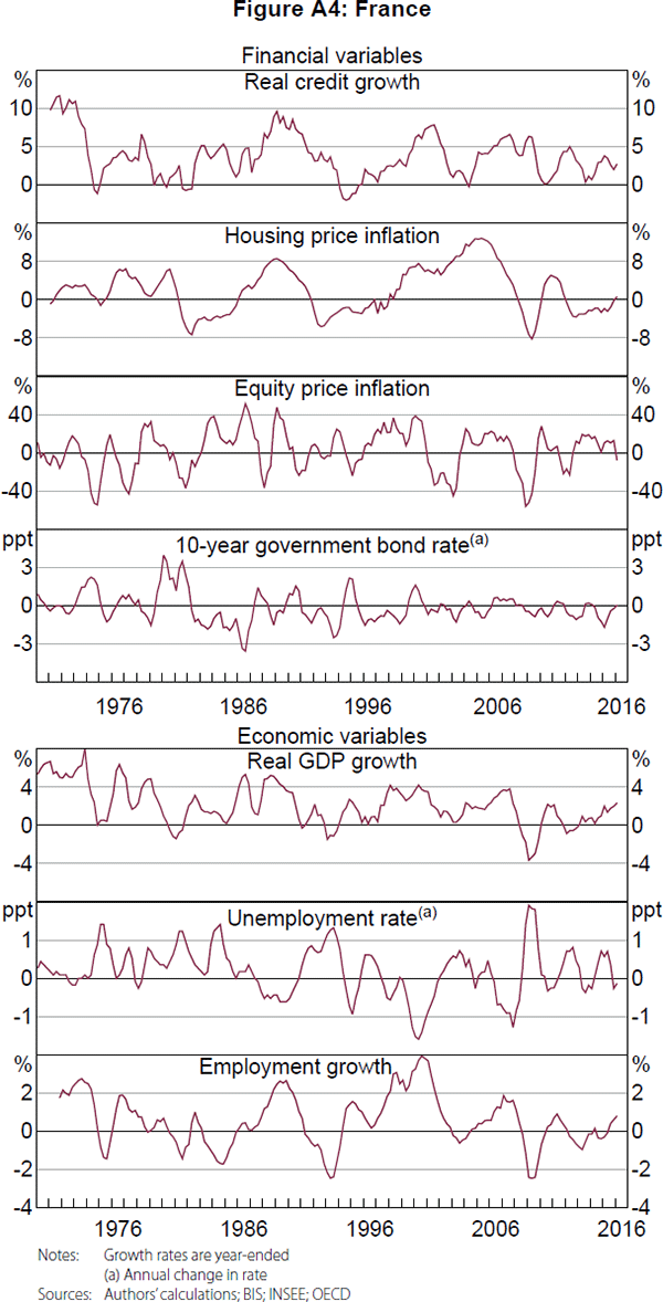
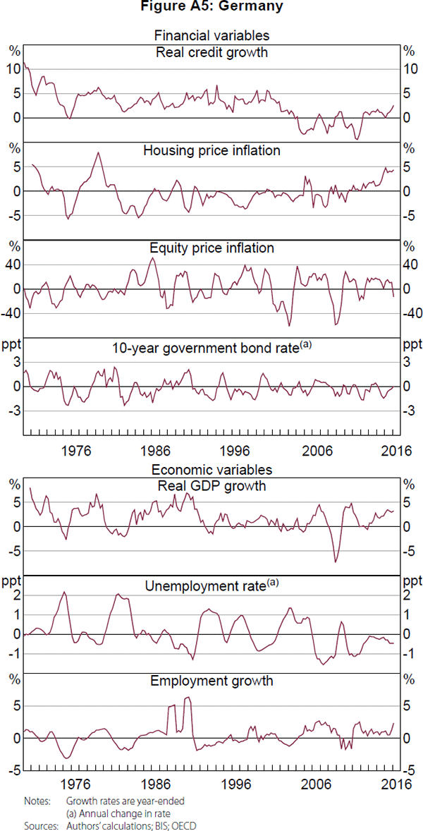
Five countries are included in our analysis: the United States, the United Kingdom, Australia, France and Germany. These countries were chosen to facilitate a comparison with the findings in the literature as well as to provide a comparison across advanced economies.
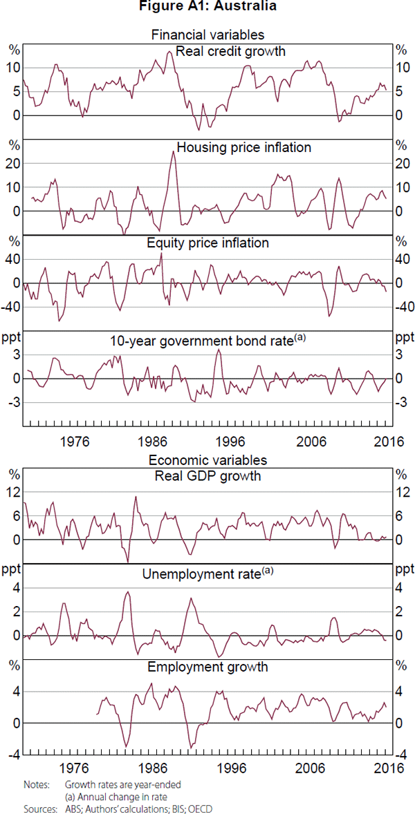
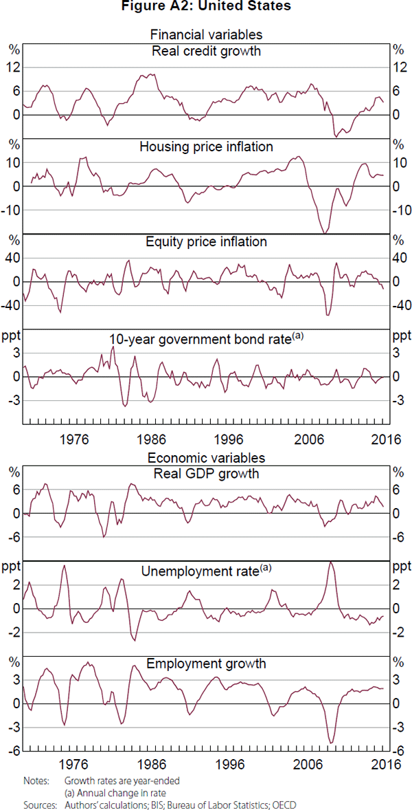
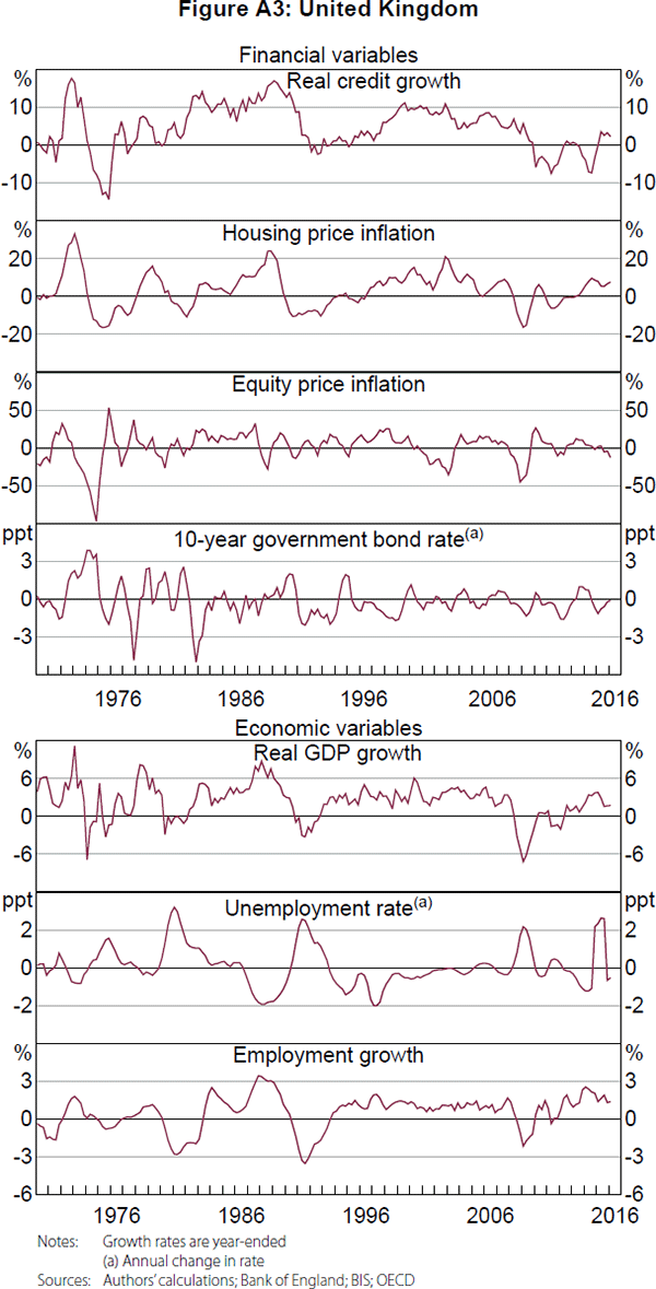
A summary of the data is presented in Table A2, and the data are shown in Figures A1–A5. The summary statistics are broadly consistent across countries, which is not surprising given the similarities between the countries. However, Germany appears to be somewhat of an outlier, with negative average house price inflation and weaker credit growth over the past couple of decades. On visual inspection, credit growth and housing price inflation generally appear to have had larger and longer cycles compared with equity price inflation and the change in government bond yields, which is a common finding in the literature (Drehmann et al 2012; Strohsal et al 2015, Schüler et al 2017). There also appear to be cycles in the macroeconomic variables.
3.3 Methodology
As discussed in Section 2, several papers approach the question of whether there is a longer financial cycle by imposing ex ante assumptions on the cycles in the data. We use two methods that do not impose such assumptions. The first method is multivariate spectral analysis, which decomposes the cross-covariance of stationary time series into different cycle frequencies. The second method is the turning point algorithm developed in Bry and Boschan (1971), which has been extended to quarterly data in Harding and Pagan (2002) and to multiple variables in Harding and Pagan (2006). It is worth noting that, as in many existing papers, we estimate these cycles separately and, as a result, we are treating the cycles as if they are separate from each other. If they are related, a better approach might be to estimate the cycles simultaneously; however, we leave this for future work.
For the first method, the frequency with the greatest contribution to the cross-covariance is considered to be the dominant cycle length at which the time series co-move. The dominant cycle in the financial variables is used as an approximation of the financial cycle, and the dominant cycle in the real economic variables is used as an approximation of the business cycle. To do this, we follow Schüler et al (2017) and calculate a measure of the multivariate spectral density called the power cohesion:
where t = 1, …, T reflects the time dimension, M reflects
the number of stationary variables in the matrix X, which is a
T × M matrix, and
ω ∈[−π,π] reflects the cycle frequency.
The function  represents the cross-spectral densities for each
pair of variables in X, with
represents the cross-spectral densities for each
pair of variables in X, with  and
and  representing the standard deviations for variables a
and b,
representing the standard deviations for variables a
and b,  rep res enting the cross-spectrum for variables
a and b, and Cov[xa,t, xb,t
+ k] representing the cross-covariance between leads and lags
of these variables; i is the imaginary unit. In our analysis, we have two
X matrices, one for financial variables and another for economic variables.
The dominant cycle is determined by finding the frequency, ω, at which PCohX
(ω) is at its maximum. To determine whether these dominant cycles are
different, we estimate a 95 per cent confidence interval for the dominant cycle frequencies
using a parametric bootstrap method.[7]
rep res enting the cross-spectrum for variables
a and b, and Cov[xa,t, xb,t
+ k] representing the cross-covariance between leads and lags
of these variables; i is the imaginary unit. In our analysis, we have two
X matrices, one for financial variables and another for economic variables.
The dominant cycle is determined by finding the frequency, ω, at which PCohX
(ω) is at its maximum. To determine whether these dominant cycles are
different, we estimate a 95 per cent confidence interval for the dominant cycle frequencies
using a parametric bootstrap method.[7]
There are two main limitations with using multivariate spectral analysis. Due to the volatility in the multivariate spectral density, we use a Parzen window to smooth the cross-spectral densities; while this could potentially compromise our results, we note that it is commonly used in the literature (e.g. Aikman et al 2015; Schüler et al 2017) and changing the bandwidth (or removing the smoothing window altogether) does not change our main conclusions. Another limitation with multivariate spectral analysis is that it requires stationarity and therefore we are only able to identify cycles in growth rates rather than classical cycles. It could also be a concern that we include both stock variables (credit) and flow variables (GDP) in our analysis and this could somehow influence our results. In Appendix B, we show that the spectral densities for a stock and its flow should be the same, though there is a phase shift between the stock and the flow.
To crosscheck the results from the multivariate spectral analysis, we use the Bry-Boschan quarterly algorithm to estimate the average duration of cycles in financial variables and in real economic variables. This algorithm identifies the peaks and troughs in a time series given specific censoring parameters, such as the minimum length of a peak, expansion and contraction.[8] This method has the advantage of being able to estimate classical cycles, rather than cycles in growth rates. However, it is not without its disadvantages; it is a purely statistical measure, with no underlying economic theory and it can be sensitive to the choice of censoring parameters.
If there is a financial cycle that is different in length from the macroeconomic cycle, as suggested in the literature, we would expect to find little overlap in the confidence intervals for the dominant frequencies for financial variables and economic variables in the multivariate spectral analysis. We would also expect to find large differences in the average duration of cycles in financial and economic variables as determined by the multivariate Bry-Boschan turning point algorithm.
Turning to how the financial and business cycles might be related, we first identify how often cycles in financial and economic variables are synchronised. For simplicity, we use credit growth to represent financial variables, and GDP growth to represent economic variables. To obtain the cycles in these variables we use a Christiano-Fitzgerald band-pass filter.[9] Using this filter, we extract two cycles from each time series: a longer cycle between 8 and 30 years, often described as the range for the length of the financial cycle in the literature, and a shorter cycle between 2½ and 8 years, often described as the range for the length of the business cycle in the literature. We use the Bry-Boschan quarterly turning point algorithm on these cycle estimates to determine the degree of synchronisation between the cycles.[10] It is important to note here that we are not assuming that we know the true length of the financial cycle or business cycle; instead, we are trying to understand how often cycles in the economy and the financial system might be in conflict. If cycles in credit growth are independent from cycles in GDP growth, or there is a significant phase shift between these cycles, we might expect the cycles to have a low degree of synchronisation.
Following this, we explore the lead/lag relationship between the identified cycles in credit and GDP growth. In particular, we employ cross-correlograms, cross-spectral densities and Granger causality tests to understand the relationship between these cycles. The results should help identify which cycle, if any, tends to lead the other at different frequencies as well as the number of lags involved. Given the discussion in the literature of a long financial cycle that leads to economic instability, credit growth could lead GDP growth at longer frequencies. At the same time, as discussed at the beginning of the paper, we expect that economic conditions matter for financial conditions and so GDP growth may also lead credit growth.
3.4 Results
3.4.1 Is there a financial cycle separate from the business cycle?
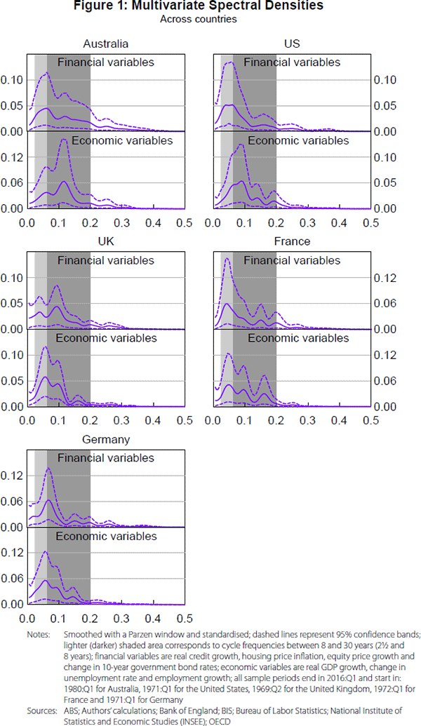
Figure 1 shows the measures of co-movement between the financial variables and between the economic variables in the frequency domain for all five countries, while Table 1 presents the estimates of the dominant cycle lengths (at which most of the co-movement occurs) and the 95 per cent confidence intervals around these estimates. These estimates are used as an approximation for the length of the financial and business cycles.
The results suggest that the length of the common cycle in financial variables is different from the length of the common cycle in economic variables. For the United States, Australia and France, financial variables tend to co-move most at longer frequencies compared with economic variables; this is consistent with the literature that claims that financial cycles are longer than the business cycle, though the estimates of the length of the financial cycle are at the lower end of the range of the estimates reported in the literature. In contrast, financial variables in the United Kingdom and Germany tend to co-move most at shorter frequencies compared with economic variables. In several countries there is a secondary peak in the multivariate spectral density for economic variables and, to some extent, financial variables, which could suggest the presence of other cycles in the data that are less dominant but are nonetheless still important.[11]
| Financial cycles | Business cycles | ||||
|---|---|---|---|---|---|
| Years | 95% confidence intervals | Years | 95% confidence intervals | ||
| Australia | 8.1 | [2.9, 18.1] | 4.3 | [3.3, 14.5] | |
| United States | 8.2 | [5.3, 22.6] | 5.7 | [4.3, 11.3] | |
| United Kingdom | 5.2 | [4.5, 47.0] | 8.5 | [4.7, 13.4] | |
| France | 12.6 | [3.4, 17.7] | 9.8 | [3.1, 17.7] | |
| Germany | 7.5 | [5.7, 22.6] | 9.1 | [4.8, 22.6] | |
|
Sources: ABS; Authors' calculations; Bank of England; BIS; Bureau of Labor Statistics; INSEE; OECD |
|||||
As a comparison to the estimates obtained using multivariate spectral analysis, we also estimate the average duration of cycles in financial and economic variables over the same time periods using the multivariate Bry-Boschan turning point algorithm. The results are presented in Table 2. In most countries, the differences between the average duration of cycles in financial variables are similar to that of economic variables.
| Financial variables(a) | Economic variables(b) | ||||||
|---|---|---|---|---|---|---|---|
| Contraction | Expansion | Cycle | Contraction | Expansion | Cycle | ||
| Australia | 3.8 | 2.0 | 5.7 | 1.3 | 5.1 | 6.4 | |
| United States | 2.2 | 3.8 | 6.0 | 1.7 | 4.5 | 6.8 | |
| United Kingdom | 1.8 | 6.4 | 8.3 | 1.2 | 5.3 | 6.5 | |
| France | 1.3 | 5.0 | 6.3 | 1.3 | 4.3 | 5.6 | |
| Germany | 2.2 | 2.4 | 4.8 | 1.9 | 3.5 | 5.5 | |
|
Notes: (a) Includes credit, housing prices, equity prices and 10-year
government bond rates Sources: ABS; Authors' calculations; Bank of England; BIS; Bureau of Labor Statistics; INSEE; OECD |
|||||||
While the multivariate spectral densities are visually different, the large confidence intervals around the estimates for financial and business cycles and the considerable overlap between these confidence intervals cast uncertainty on the true cyclical behaviour of financial and economic variables. Given the overlap between the confidence intervals as well as the results from the turning point method, we cannot confidently conclude from our analysis that the financial cycle is longer than the business cycle.
There are some weaknesses in our analysis that could affect the results. The first is that structural breaks may have occurred, leading to changes in the cycles over time; this is plausible given that our results cover a time period in which political and economic policy regimes changed significantly, including the reunification of Germany, financial liberalisation and changes in monetary regimes. The turning point method results should provide some robustness here, since the time-varying nature of this method implies that it would be less affected by structural breaks than spectral analysis. As an additional robustness check, we repeat the multivariate spectral analysis using data from 1980 onwards for all countries (Table C1).[12] While the change in sample periods does affect the results to some extent, particularly for the United States and the United Kingdom, the confidence intervals around our estimates remain wide and still overlap.
Secondly, our choice of financial variables could influence our results. As documented in the literature, there appears to be a consensus that credit growth and housing price inflation are more relevant when it comes to measuring the financial cycle than other financial variables, reflecting their superior ability to predict financial crises (Drehmann et al 2012; Jordà et al 2015). As a robustness check, we repeat our analysis excluding equity prices and the long-term government bond rate. As shown in Tables C2 and C3, excluding these variables leads to an increase in the dominant cycle lengths in the multivariate spectral densities for financial variables. Also, for the United States and France, this leads to an increase in the average duration of the cycles in financial variables from the multivariate Bry-Boschan turning point algorithm. Nonetheless, there remains a significant overlap in the confidence intervals around the dominant frequencies in the multivariate spectral densities for financial and economic variables, and the turning point method still estimates similar cycle lengths for some countries. Therefore, we believe that there is still insufficient evidence to conclude that the financial cycle is longer than the business cycle.
Finally, there is the issue of insufficient data. If, as claimed by other papers, there exists a longer financial cycle and we have data covering less than five decades, there will only be a limited number of cycles in the data and it will be difficult to confidently identify the length of the cycle. As another robustness check, we repeat the multivariate spectral analysis using the long-run annual database provided by Jordà, Schularick and Taylor (2017).[13],[14] The results are provided in Table C4. These results are not entirely consistent with the quarterly data, particularly for the United Kingdom and Australia, which is unsurprising given that the annual data cover a much longer time period than the quarterly data and many structural breaks are likely to have occurred over this period. Notably, the confidence intervals remain large around the dominant frequencies for financial and economic variables, implying that, even with a longer dataset, we cannot verify that the financial variables have a different cycle length to economic variables.
Given that the robustness checks do not provide evidence that cycles in financial variables differ considerably from cycles in economic variables, we conclude that our results do not provide sufficient evidence for the existence of a financial cycle that is longer than the business cycle. This is not to say that this claim cannot be true, but rather that we cannot find enough evidence to support this claim.
3.4.2 How are the financial variables and business variables related?
Despite the fact that we do not have evidence that the length of cycles in financial variables and economic variables differ considerably, it is still important to understand the relationship between these cycles. It is possible that these cycles have different lengths but we cannot prove it due to a lack of data, meaning that there would undoubtedly be times that they are in different phases of the cycle; and, even if they are similar in length, they could be in different phases at the same time. In fact, just observing current and recent events across many countries suggests that developments in financial variables can be at odds with developments in economic variables. If there is a relationship between these cycles, knowing how often the cycles are in the same phase will be useful to help understand how often there might be conflict between the cycles (and the policies that manage them).
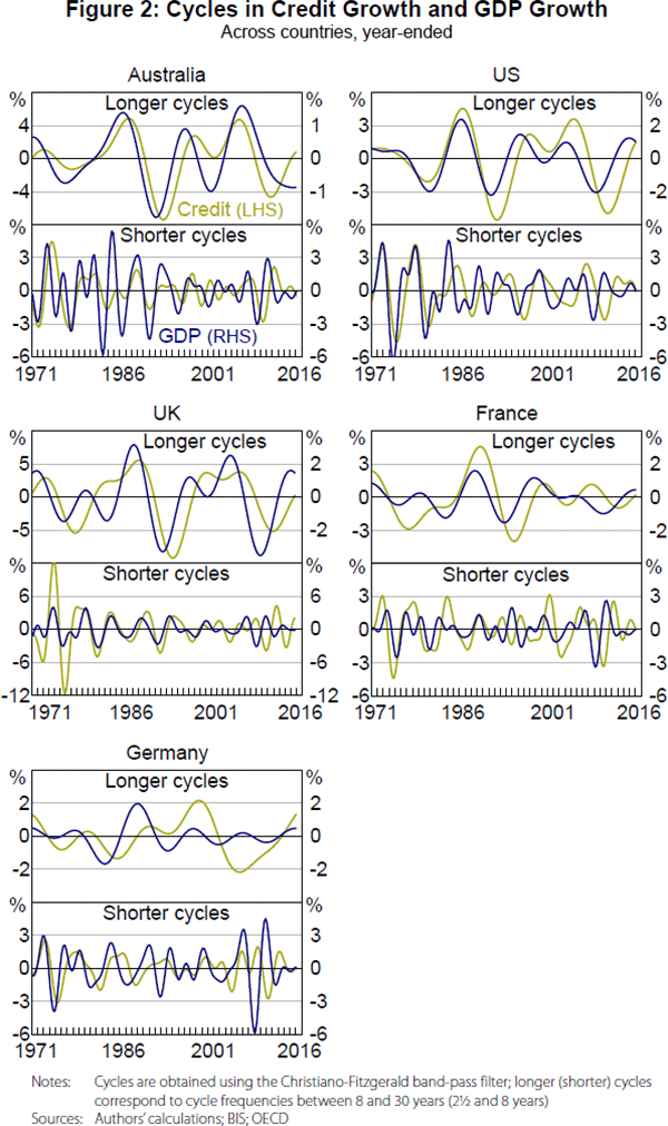
Figure 2 presents the estimated cycles in credit growth and GDP growth across the five countries, using the Christiano-Fitzgerald band-pass filter; the longer and shorter cycles shown in this figure correspond to cycles of 8 to 30 years and 2½ to 8 years, respectively. It is clear that the cycles in credit growth and GDP growth are similar, though they are sometimes out of sync, and it looks as though these cycles are related. The longer cycles in credit growth and GDP growth appear to be particularly synchronised in the United States and Australia.
Using the Bry-Boschan turning point algorithm updated in Harding and Pagan (2002), Table 3 presents the average duration of contractions and expansions in the longer and shorter cycles in credit and GDP growth, as well as the degree of synchronisation between these cycles. The length of expansions and contractions are similar for the cycles in credit and GDP growth, suggesting a similar length in the cycles.
| Credit growth | GDP growth | Degree of synchronisation Concordance statistics | ||||
|---|---|---|---|---|---|---|
| Contraction | Expansion | Contraction | Expansion | |||
| Longer cycles | ||||||
| Australia | 4.8 | 6.1 | 5.2 | 5.2 | 0.73 | |
| United States | 5.8 | 4.4 | 4.4 | 4.3 | 0.77 | |
| United Kingdom | 5.0 | 4.2 | 5.0 | 4.7 | 0.57 | |
| France | 4.3 | 4.7 | 4.7 | 4.3 | 0.65 | |
| Germany | 5.1 | 4.4 | 6.2 | 4.6 | 0.64 | |
| Average | 5.0 | 4.8 | 5.1 | 4.6 | 0.67 | |
| Shorter cycles | ||||||
| Australia | 1.6 | 1.5 | 1.8 | 1.5 | 0.61 | |
| United States | 2.3 | 1.7 | 2.2 | 1.8 | 0.55 | |
| United Kingdom | 2.3 | 1.9 | 2.1 | 1.9 | 0.60 | |
| France | 1.7 | 1.5 | 1.8 | 1.6 | 0.51 | |
| Germany | 1.9 | 1.9 | 2.1 | 2.1 | 0.54 | |
| Average | 2.0 | 1.7 | 2.0 | 1.8 | 0.57 | |
|
Notes: Longer (shorter) cycles correspond to cycle frequencies between 8 and 30 years (2½ and 8 years); concordance statistics represent the proportion of time the cycles are in the same phase Sources: Authors' calculations; BIS; OECD |
||||||
In terms of synchronisation, the longer cycles in credit and GDP growth have a higher degree of synchronisation, compared with the shorter cycles in credit and GDP growth. Compared with two random series, which you would expect to be in sync 50 per cent of the time, the longer cycles were in sync 67 per cent of the time on average across the countries, while the shorter cycles were in sync 57 per cent of the time.[15] For the United States and Australia, the longer cycles are in sync for around three-quarters of the time. The high degree of synchronisation between the cycles in the United States and Australia could reflect the importance of the financial services sector to their economies, though it is interesting that we do not find a similar result for the United Kingdom, which also has a large financial sector. In addition to looking at synchronisation within countries, we can also estimate the degree of synchronisation across countries. Table D1 presents these results and shows that the cycles across countries can be reasonably synchronised, which could mean that the cycles are influenced by international developments as well as domestic factors.
While the cycles in credit and GDP growth have often been in the same phase, there have still been times when they are in different phases. What this means for policymakers depends on the relationship between the cycles. The literature discussed in Sections 2 and 3.1 provides many reasons why a relationship may exist between developments in the financial system and the economy. If we do find evidence of a relationship, developing a better understanding of this relationship should help policymakers to forecast the future paths of the cycles in credit and GDP and set policy accordingly.
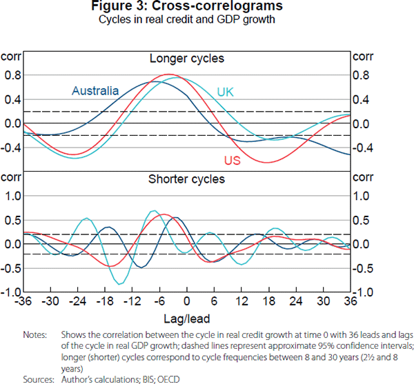
A visual inspection of the time series estimates of the cycles suggests that cycles in credit and GDP growth are related. This can also be seen in the cross-correlation between the cycles. In general, we find that lags in the cycles of GDP growth are positively correlated with the cycles in credit growth up to a few years ahead, particularly for the longer cycles (Figure 3).[16] This suggests that cycles in GDP growth could positively lead cycles in credit growth. At the same time, some longer leads/lags in GDP growth cycles are negatively correlated with credit growth cycles. This suggests that cycles in credit growth could negatively lead cycles in GDP growth. Therefore, the relationship could run both ways, or there could just be a one-way relationship with a phase shift.
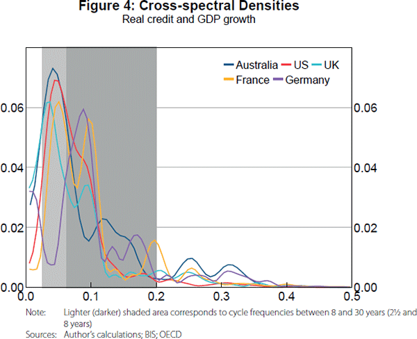
Moving from the time domain to the frequency domain, Figure 4 presents cross-spectral densities for credit and GDP growth, which are effectively decompositions of the cross-correlation between the cycles in the frequency domain. The co-movement between credit and GDP growth appears to be strongest at lower frequencies; that is, credit and GDP growth tend to co-move more in the longer run. The exception here is Germany, where a significant amount of cross-correlation occurs at frequencies between 2½ and 8 years. Using the phase spectrum, we can determine the lead/lag relationship between credit and GDP growth at different frequencies.[17] While the phase spectrum can often be difficult to interpret, our results suggest that credit growth tends to lead GDP growth at longer frequencies.
So far, we have only looked at the correlation between the cycles; this does not prove (nor rule out the possibility of) a relationship between credit and GDP growth. Assuming a relationship does exist and abstracting from other variables relevant in this relationship, there are two plausible cases of a causal relationship occurring between credit growth and GDP growth that are consistent with our results and the theory:
- GDP growth → credit growth. Changes in GDP growth are independent from changes in credit growth and cause changes in credit growth. The ability of GDP growth to affect credit growth is intuitive in terms of economic theory and is suggested in the results above. In this case, GDP growth leads credit growth and the negative correlation between credit growth and the longer leads/lags of GDP growth merely reflects the same relationship but with a phase shift.
- Credit growth ↔ GDP growth. As discussed earlier in the paper it is also entirely reasonable to expect that credit growth can influence GDP growth and this could help to explain some of the results from the cross-correlograms and cross-spectral densities. There is potential for both a positive and negative relationship to exist. For example, a strong rise in credit growth may be associated with a build-up in risks that, if they materialise, could significantly affect the financial system and the economy. There is also the potential for positive effects for the economy during these expansions, including the extension of credit to productive and innovative ventures.
To formally test whether the relationship is one-way, or whether it runs both ways, we employ Granger causality tests. Table 4 presents the p-values from the tests for whether GDP growth Granger causes credit growth and vice versa.[18] Overall, the results suggest that cycles in GDP growth Granger cause cycles in credit growth in all countries. For some countries, there is evidence that cycles in credit growth and GDP growth Granger cause each other, suggesting that the relationship could run both ways.
| Alternative hypothesis | Australia | United States | United Kingdom | France | Germany |
|---|---|---|---|---|---|
| Actual data | |||||
| Credit growth → GDP growth | 0.04 | 0.14 | 0.75 | 0.06 | 0.29 |
| GDP growth → credit growth | 0.03 | 0.03 | 0.01 | 0.04 | 0.13 |
| Longer cycles(a) | |||||
| Credit growth → GDP growth | 0.06 | 0.05 | 0.39 | 0.24 | 0.01 |
| GDP growth → credit growth | <0.00 | <0.00 | <0.00 | <0.00 | <0.00 |
| Shorter cycles(a) | |||||
| Credit growth → GDP growth | 0.01 | 0.18 | 0.23 | 0.58 | 0.09 |
| GDP growth → credit growth | 0.10 | 0.06 | <0.00 | <0.00 | 0.08 |
|
Note: (a) Granger causality tests were not possible with the data filtered using a band-pass filter, so these cycles are identified using an HP filter with lambda chosen by optimising the spectral density of the actual series between 8 and 30 years for longer cycles and 2½ and 8 years for shorter cycles Sources: Authors' calculations; BIS; OECD |
|||||
Overall, it is clear that there is some lead/lag relationship between credit and GDP growth. The results suggest that GDP growth leads credit growth, but at the same time they do not rule out the possibility that credit growth leads GDP growth. The mixed results imply that we cannot confirm whether the cycle in financial variables leads or lags the cycle in economic variables in the long or short run. In a way, the mixed results are not surprising given the discussion on the links between the financial system and the economy at the beginning of this paper. It is likely that the relationship between credit and GDP growth depends on the circumstances and other factors not captured in this analysis, meaning that in some cases GDP growth will lead credit growth and in other cases credit growth will lead GDP growth. The interpretation of these results is further complicated by the potential for regime switching, for example, due to the presence of the financial liberalisation in the data. However, what is clear from our results is that the cycles are unlikely to be independent of each other and will sometimes be moving in different directions.
4. Policy Implications
The analysis presented in this paper suggests that there is little evidence to conclude that cycles in financial and economic variables operate at different frequencies – in particular, it is difficult to argue that financial variables have a cycle that is longer than the cycle in economic variables. It is worth noting, however, that we cannot definitively conclude that these two cycles have the same frequency and the results may be subject to type II error (failure to reject the null hypothesis that the peak frequencies are the same when they are, in fact, different). Furthermore, the evidence suggests that developments in economic variables lead those in financial variables, but it is more difficult to conclude the converse. While the power of these tests may not be high, the results suggest that much more evidence is required to establish whether the cycles in these variables are distinct from one another, and if so, why that might be the case.
Unfortunately, our analysis, and those of many other authors, does not give us any insights into what drives these cycles and the mechanisms through which the two cycles affect each other. These are important considerations if we are going to draw some policy implications. Since we are unable to identify the drivers of these cycles, we are limited to considering general scenarios of how they may relate to each other.
It is highly unlikely that the two cycles are independent of each other and have similar frequencies by chance. It is very likely that if the two cycles have a similar frequency, they also have common drivers. As a result, financial variables should be useful in understanding developments in the business cycle.
If the main drivers of the two cycles were real (e.g. productivity), then fluctuations in financial variables, particularly credit, would reflect fluctuations in the need to finance economic activity. Financial variables would be used by policymakers to make an inference about the state of the economy. In this view of the world, the standard policy tools that have typically been used to address cyclical fluctuations in activity, namely fiscal and monetary policy, would continue to be used to ‘smooth’ out the business cycle and minimise variations in GDP growth and unemployment, and minimise deviations of inflation from its target. The extent to which fluctuations in each are tolerated will depend on the weights placed on these elements in the policymakers' loss function. Policymakers would only be concerned with, and respond to, fluctuations in financial variables to the extent that these variables are informative about economic conditions.
However, some have argued that the conduct of monetary policy can contribute to the cycles we observe in financial variables (Borio 2012; Juselius et al 2016). Borio argues that monetary policy that is too narrowly focused on inflation may not necessarily tighten policy when financial ‘booms’ occur because inflation is low and stable. This paper suggests a scenario where the potential growth rate of the economy rises, causing credit growth and asset price inflation to rise, but the spare capacity in the economy constrains the monetary authority's ability to respond. We do not find this scenario convincing. The cause of the increase in potential growth matters. If the potential growth rate of the economy increased due to a rise in productivity growth, this would raise the neutral real interest rate in the economy, and soon enough the monetary authority would realise the need to begin to tighten monetary policy, which would reign in any boom in credit and asset prices.
It is possible, however, that some drivers of these cycles could be financial rather than real in nature; that is, drivers that are specific to the financial system and independent of economic conditions. In this case, there could be grounds for policymakers to address cyclical fluctuations in both economic and financial activity. The key question is what these drivers could be.
Many of the financial drivers identified in the literature relate to sentiment, particularly regarding risk, and expectations (especially for asset prices).[19] One mechanism by which a financial cycle can affect the business cycle is through changes in the perception of risk that can affect the propensity for agents to underestimate the risks that they are taking during economic expansions. This leads to agents taking on more risk than they would otherwise, which can be reflected both in the type of investments or portfolio allocations they make and in the amount of leverage they are willing to use to fund these activities. This can be reflected in ‘overvalued’ assets, expectations of sustained higher asset price inflation, unsustainable levels of debt and lower credit spreads and can, ultimately but not always, lead to higher loan defaults and a contraction in bank lending that results in a contraction of economic activity. This is not to say that it is just households and firms that take these risks; the financial sector can also underestimate risks that lead to imprudent management of its balance sheet. Once growth slows, or a recession begins, perceptions of risk adjust and could even lead to agents overestimating risk, leading to higher spreads and expectations of asset price deflation that can exacerbate the amplitude of the business cycle. The main question is: what causes these changes in perceptions of risk and expectations of asset price inflation? It seems likely that real shocks to the economy will play an important role here.
If there are financial drivers, the business and financial cycles may sometimes be in different phases. In particular, there will be times when the economy is slowing (including the case where growth is positive but below potential) but there is reasonably high asset price inflation and accelerating credit. This raises the question of how to deal with such situations, whether it should be dealt with at all, and if so, what are the appropriate policy tools to address this confluence of events. The main research questions, which we do not address here, are: what are the market distortions and potential market failures that lead to this, admittedly infrequent, confluence of events? Why would agents continue to borrow (presumably unsustainably)? Why would the financial system continue to lend in this environment? Why are some asset prices not responding to slower growth in the economy? In a first-best world where we understand the answers to these questions and are unconstrained, we would be able to design policies to address the distortions and market failures that produce these outcomes. However, this is not always the case and so we focus on the role of policy in addressing the symptoms of these distortions and market failures, which we refer to as ‘financial imbalances’.
4.1 Monetary policy and the financial cycle
Monetary policy has traditionally been used to deal with the business cycle. It is particularly good at doing this because interest rates provide the price signal for agents to intertemporally reallocate resources; during booms, interest rates rise and encourage agents to push economic activity into the future, while during downturns rates are lowered and encourage agents to bring economic activity forward from the future. Monetary policy does this to both keep unemployment around the non-accelerating inflation rate of unemployment and inflation around its target. However, by adjusting interest rates, monetary policy also has an effect on credit growth and asset price inflation. So if the economic conditions and inflation warrant lower interest rates but credit growth and asset price inflation are still ‘too high’, should monetary policy be used to curtail the potential risks this might pose to economic activity in the future?
Traditionally, the policymaking framework has focused on the role of monetary and fiscal policy to moderate the business cycle, and prudential policy to address the risks in the financial system.[20] The risks discussed in the financial cycle literature do not just consider the risks on financial institutions' balance sheets, but also the risks on private sector non-financial balance sheets. These risks can be magnified by asset prices that are too high and inflating at a rapid rate, and credit growing at an ‘unsustainable’ pace.
A laissez-faire view of this problem is that markets are efficient and that households and firms know the risks they are taking; they will bear the consequences if those risks materialise. Therefore, to the extent that these risks are idiosyncratic and uncorrelated, and that prudential policy has been applied appropriately, there is no need for further policy intervention. Another argument, however, is that these risks across households and firms are correlated, and that externalities related to a number of households and firms experiencing financial distress at once are large and negative – those who were more prudent in their decision-making would still be affected if these risks materialised. Under such a scenario, there should be a policy intervention to ensure that these particular risks are managed appropriately and that the consequences of such a scenario are minimised.
The conundrum for monetary policy is that there are a number of channels by which it can affect risk-taking behaviour. Lower interest rates can encourage banks to take on more risks such as higher leverage, greater maturity mismatch and easier lending standards (Gambacorta 2009; Agur and Demertzis 2015). Lower interest rates can also encourage investors to ‘search for yield’ and to expose themselves to more risk (Rajan 2005). Together, these are often referred to as the ‘risk-taking channel’ of monetary policy (Borio and Zhu 2012; Bruno and Shin 2015). In addition, higher asset prices resulting from lower rates increases the value of collateral, potentially encouraging greater borrowing and creating an asset price boom fuelled by credit. Alternatively, higher interest rates increase debt repayment burdens, which can potentially lead to higher default rates (Sengupta 2010). Higher interest rates also put pressure on banks' funding costs, thereby compressing their profit margins and potentially encouraging them to engage in riskier lending (Agur and Demertzis 2015). Exchange rate appreciations associated with interest rate increases can encourage foreign currency borrowing, which can pose significant risks to unhedged foreign currency borrowers during any subsequent depreciation.
Agur and Demertzis (2015) finds that the ‘risk-taking channel’ tends to dominate banks' risk-taking behaviour during the upswing of a financial cycle, while the profitability channel tends to dominate during the contraction phase. Drawing on this result, the scenario outlined above where the macroeconomy is in a contractionary phase but the financial cycle is in an expansionary phase would put some pressure on the central bank to ease policy, but this could encourage more risk-taking at a time when these risks may already be unacceptably high. The choice a central bank makes in this situation will depend on how much value it places on achieving its objectives in the long term versus the short term. In the case of an inflation-targeting central bank, the other consideration would be the effect on inflation expectations, as a protracted deviation from the inflation target could lead to a shift in expectations and therefore make the inflation objective harder to achieve in the long term.
Despite the potential for short-term conflict, in the long run price stability should have some positive spillovers for financial stability, and vice versa, since a stable macroeconomic environment and a stable financial environment are necessary conditions for each other (Smets 2013). Furthermore, to the extent that easier monetary policy can raise inflation and nominal income growth, this should help reduce the debt repayment burdens for borrowers. Also, during a downturn, some risk-taking may be desirable to encourage more investment and growth. The difficulty for central banks is determining what amount of risk is desirable and when those financial risks become material enough to potentially pose a threat to macroeconomic stability. This is where prudential policy plays an important role. Smets (2013) and Maddaloni and Peydró (2013) find evidence that the effect of lowering interest rates on banks' risk-taking is reduced under more rigorous prudential policy. Therefore, one avenue to manage these risks is through prudential policy.
This begs the question as to what instruments should be used to address price and economic stability, and whether we can rely on one instrument to manage the business and financial cycles (assuming there are times they are in conflict). Tinbergen (1952) suggests that the number of policy instruments that should be used is the same as the number of policy objectives. Policy instruments should be used to achieve the objectives they can most efficiently attain. This principle would suggest that monetary policy should focus on targeting price stability, where it has been proven effective, and leave other instruments to target other policy objectives. Since the nominal interest rate is only one tool, can it be expected to effectively achieve its traditional objectives in addition to managing the financial cycle?
4.2 Macroprudential policy
Due to the blunt nature of monetary policy, many papers have concluded that using it to target concerns regarding risks to the financial system would require large changes in interest rates, which would be costly and inefficient, particularly when the risks are building up in a specific area of the financial system (e.g. Alpanda, Cateau and Meh 2014; Svensson 2016). In contrast, macroprudential policy consists of a range of tools, which means it can have greater flexibility to manage specific risks and allow monetary policy to focus on its primary objectives. The most common macroprudential tools include: caps on loan-to-valuation ratios (LVRs); minimum serviceability requirements; and capital requirements. These tools can be targeted to address the build-up of risks for particular sectors – such as the household sector – and strengthen the financial system's resilience.
It is unlikely that macroprudential policy is capable of perfectly addressing all types of risks that build up during the expansionary phase of a financial cycle. One clear side effect of using macroprudential policy to restrict lending to a particular sector of the economy is the diversion of borrowers to unregulated financial institutions (the shadow banking system) where policymakers tend to have limited influence; in this case, a blunt tool such as monetary policy could be more effective by controlling the cost of funds (according to Stein (2013), monetary policy ‘gets in all of the cracks’).
Another drawback is the uncertainty around the effectiveness of some macroprudential tools. The effectiveness is likely to vary depending on the type of tool used and the circumstances in which it is used (Cerutti, Claessens and Laeven 2015). Moreover, it can be difficult to measure the effectiveness of macroprudential tools for a number of reasons, including the lack of a clear and quantifiable target and limited experience with using these tools in the post-crisis period. Furthermore, it is not entirely clear under what circumstances these instruments would be effective and when they would be ineffective. For example, Guibourg et al (2015) suggests that countercyclical capital requirements would not have been sufficient to stop rapid credit growth in the lead-up to the financial crisis in the United Kingdom and Spain.
There are also significant institutional issues related to macroprudential policy. For the macroprudential tools to be a useful part of the policy arsenal, it must be clear that they can be used without political interference. That is, the responsible authority must have the independence to use the tools at its disposal. There is the question of who should be in control of these instruments, particularly when the financial regulator and central bank are separate. Macroprudential policy determined by the central bank would require the financial regulator to implement these policies. It would be unclear, in this instance, which institution would be accountable for the use of the tools. Finally, there is a question as to how quickly some policies can be implemented and enforced – if the time required is too long, risks may have materialised before the policies can be implemented, by which time the policies may need to be abandoned.
The other drawback of trying to use macroprudential tools to manage financial risks in the economy is that they could alter the risk profile of projects being undertaken as lending to the private sector becomes a binding constraint on economic activity. While these policies may be effective, they can be just as blunt as monetary policy. This means that some viable, albeit riskier, investments may be denied funding, which could result in less funding for innovation that would have otherwise helped to drive higher productivity growth.
4.3 Implications for monetary policy
Despite these potential limitations and costs, macroprudential policy would still be a valuable complement by helping to manage some risks as monetary policy tries to stabilise economic activity. This means that we need to consider how monetary and macroprudential policies might interact. These policies should move together and reinforce each other when the cycles are in sync. However, when the business and financial cycles are out of sync, these policies may pull in different directions and counteract the effect of the other. We know from the previous section that the stance of monetary policy can influence the build-up of risks and therefore the appropriate stance of macroprudential policy. What is of interest in this section is how changes in macroprudential policy, responding to a change in financial imbalances either related or unrelated to the stance of monetary policy, will affect the transmission of monetary policy.
To some extent, this type of discussion is not new; there has been extensive research on the interactions between policies, most notably monetary and fiscal policy (the most obvious example being Sargent and Wallace (1981)). In the case of monetary and fiscal policy, both policies arguably target the business cycle and therefore have similar objectives; however, these policies have different tools and any conflict tends to come from political constraints.
We expect there to be some overlap in transmission channels between monetary and macroprudential policies since both policies work to achieve their objectives by affecting the price and quantity of credit in the economy as well as asset prices. The extent to which the interactions between these policies are significant will depend on the nature of the macroprudential tool that is being used (Dunstan 2014). In particular, it seems reasonable to expect that a broad-based macroprudential tool will have different implications for monetary policy than a narrow tool (i.e. one that targets a specific sector, institution or market).
Macroprudential tools that affect the distribution of credit, such as LVR limits, will likely affect the functioning of monetary policy's wealth and balance sheet channels, since these tools are most effective in tempering rapid credit and asset price growth. For example, a tightening in these tools can reduce the effect of lower interest rates on housing price inflation, which can lead to lower household consumption through the wealth effect and tighter borrowing constraints due to lower collateral values. As a result, the demand and inflation outlook is likely to be lower than if a tightening of macroprudential policy had not occurred.
Capital-based macroprudential tools can alter the price and supply of credit since equity funding is generally more expensive than debt funding (Harimohan and Nelson 2014). In response to higher capital requirements, banks have the option to increase retained earnings through lower dividend payouts, to issue new capital and pass through higher funding costs to borrowers in the form of higher lending rates, or to change the composition or size of their lending portfolio. All options can have implications for the outlook for demand and inflation; for example, changes to banks' assets could reduce the supply of credit. Higher lending rates could offset some of the effects that accommodative monetary policy has in encouraging borrowing and current consumption. Though, if banks do choose to raise new capital, it is possible that more intense competition can limit their ability to pass on higher lending rates to borrowers.
Liquidity-based tools can affect banks' holding of illiquid assets, alter credit supply (e.g. long-term lending) and, to the extent that they weigh on bank profitability, may result in higher lending rates. In addition, banks may have to change their funding profiles, which can make funding more expensive. This would also be passed on to customers (e.g. higher lending rates), which would reduce the effectiveness of monetary policy.
Overall, it appears that when the cycles are in sync, macroprudential policy should reinforce monetary policy. When the cycles are out of sync, macroprudential policy may work against monetary policy by counteracting its effects on the price and quantity of credit in the economy, and therefore domestic demand and inflation. However, this will vary depending on the type and scope of the macroprudential tools used. Some coordination of monetary and macroprudential policies will be required to ensure that all objectives can be achieved and all trade-offs are managed over an appropriate horizon.
Despite the drawbacks of macroprudential policy as well as the potential for monetary and macroprudential to interact, we believe that it is not ideal to use monetary policy to manage the financial cycle by itself; it seems reasonable to think that macroprudential policy should play a part. There are some reasonable arguments for central banks to consider their effect on financial risks when determining the appropriate course of action for monetary policy. However, we would agree with the view expressed by Peter Praet (2016) that the first line of defence must be a strong institutional and legal framework that directly targets the distortions and market failures that allow financial imbalances to occur.
5. Conclusion
Since the global financial crisis, there has been substantial work to identify the causes of the crisis and understand how future crises can be prevented. Among this work, it has been proposed, and has become commonly accepted, that there is a financial cycle that is longer than the business cycle and which should be managed separately from the business cycle. Our results suggest that there is not enough evidence to conclude that the financial cycle is longer than the business cycle. Nonetheless, even if these cycles are similar in length, there could still be reasons for policymakers to address developments in the financial system. In particular, we find that the financial and business cycles are not always synchronised and could potentially influence each other. Generally, we expect the business cycle will lead the financial cycle, but our results and observations from financial crises suggest that it is also possible for financial developments to have a significant effect on economic activity.
While the literature suggests that monetary policy does have an effect on the financial cycle, we argue that there are limitations on its ability to manage the business and financial cycles at the same time. Although it is not a perfect solution, macroprudential policy has the flexibility to help manage the financial cycle, but if it were to be used, it would need to be coordinated with monetary policy to achieve policymakers' economic and financial objectives, and to ensure that the trade-offs are being managed appropriately across all the tools being used.
What our analysis does not do, nor do many other papers, is explain the drivers of these cycles. There is a very lengthy research agenda in the profession that has tried to explain business cycles and, while our understanding has improved in this process, our knowledge is still fairly limited. If that experience is anything to go by, it will take a long time to get a decent understanding of what drives financial cycles, if they exist.
Appendix A: Data Sources
| Australia | United States | United Kingdom | France | Germany | |
|---|---|---|---|---|---|
| Credit | BIS (1953:Q4–2016:Q1) | BIS (1952:Q4–2016:Q1) | BIS (1963:Q1–2016:Q1) | BIS (1969:Q4–2016:Q1) | BIS (1948:Q4–2016:Q1) |
| Housing prices | BIS (1970:Q1–2016:Q1) | BIS (1970:Q1–2016:Q1) | OECD (1968:Q2–2016:Q1) | BIS (1970:Q1–2016:Q1) | BIS (1970:Q1–2016:Q1) |
| Equity prices | OECD (1958:Q1–2016:Q1) | OECD (1957:Q1–2016:Q1) | OECD (1958:Q1–2016:Q1) | OECD (1957:Q1–2016:Q1) | OECD (1960:Q1–2016:Q1) |
| 10-year government bond rate | OECD (1969:Q3–2016:Q1) | OECD (1953:Q2–2016:Q1) | OECD (1960:Q1–2016:Q1) | OECD (1960:Q1–2016:Q1) | OECD (1956:Q2–2016:Q1) |
| GDP | OECD (1959:Q3–2016:Q1) | OECD (1947:Q1–2016:Q1) | OECD (1955:Q1–2016:Q1) | OECD (1949:Q1–2016:Q1) | OECD (1970:Q1–2016:Q1) |
| Employment | ABS (1978:Q1–2016:Q1) | Bureau of Labor Statistics (1939:Q1–2016:Q1) | Bank of England (1950:Q3–2016:Q1) | INSEE (1970:Q4–2016:Q1) | OECD (1962:Q1–2016:Q1) |
| Unemployment rate | OECD (1966:Q3–2016:Q1) | OECD (1955:Q1–2016:Q1) | OECD (1955:Q1–2016:Q1) | OECD (1967:Q4–2016:Q1) | OECD (1968:Q4–2016:Q1) |
| CPI | OECD (1948:Q4–2016:Q1) | OECD (1955:Q1–2016:Q1) | OECD (1955:Q1–2016:Q1) | OECD (1955:Q1–2016:Q1) | OECD (1955:Q1–2016:Q1) |
| Australia | United States | United Kingdom | France | Germany | |
|---|---|---|---|---|---|
| Financial variables | |||||
| Credit growth | 5.7 (3.6) |
3.4 (3.4) |
4.6 (6.2) |
3.7 (2.9) |
2.7 (2.8) |
| Housing price inflation | 2.8 (6.4) |
1.6 (6.1) |
3.3 (9.4) |
1.9 (4.8) |
−0.3 (2.5) |
| Equity price inflation | 0.3 (19.6) |
2.2 (16.4) |
1.1 (19.2) |
2.1 (22.3) |
2.0 (20.6) |
| 10-year government bond rate (Δ4) | −0.1 (1.3) |
−0.1 (1.2) |
−0.2 (1.3) |
−0.2 (1.2) |
−0.2 (1.0) |
| Economic variables | |||||
| GDP growth | 3.1 (2.7) |
2.2 (2.5) |
2.4 (2.9) |
2.2 (2.1) |
1.8 (2.4) |
| Employment growth | 1.8 (1.6) |
1.4 (1.9) |
0.3 (1.4) |
0.6 (1.4) |
0.4 (1.6) |
| Unemployment rate (Δ4) | 0.1 (1.0) |
0.0 (1.1) |
0.1 (1.1) |
0.2 (0.6) |
0.1 (0.8) |
|
Notes: This table presents the means and standard deviation (in parentheses); all nominal variables are expressed in real terms; some variables cover shorter time periods; house price inflation data starts in 1971:Q1, with an exception for the United Kingdom; GDP growth and employment growth data for France start in 1971:Q1 and 1972:Q1, respectively; employment growth data for Australia starts in 1979:Q1 Sources: ABS; Authors' calculations; Bank of England; BIS; Bureau of Labor Statistics; INSEE; OECD |
|||||
Appendix B: Cycles in Stocks and Flows
We assume a continuous time model. All debt is taken out at time τ and is fully paid-off by period τ+T (i.e. it is T-period debt). Let Dτ (t) be the debt outstanding at time t for debt drawn down at time τ. For credit-foncier debt, the general expression for the outstanding balance of debt at time t is given by
At time t, the total outstanding stock of debt S(t) is equal to the sum of all outstanding debt drawn down between period t − T and t
Now, suppose the flow of new debt, Dτ (τ) in period τ has a cycle. So let Dτ (τ)=A sin(ατ)+B. Without loss of generality we assume that there is no phase shift.
Then it can be shown that
So S(t) has frequency  , albeit with a
phase shift.
, albeit with a
phase shift.
Details on the derivations are available from the authors upon request.
Appendix C: Robustness Checks
| Financial cycles | Business cycles | ||||
|---|---|---|---|---|---|
| Years | 95% confidence interval | Years | 95% confidence interval | ||
| Australia | 8.1 | [3.2, 24.2] | 4.3 | [3.3, 14.5] | |
| United States | 8.1 | [6.0, 36.3] | 8.1 | [4.3, 14.5] | |
| United Kingdom | 12.1 | [2.7, 36.3] | 8.1 | [4.8, 14.5] | |
| France | 10.4 | [4.8, 24.2] | 9.1 | [4.8, 72.5] | |
| Germany | 8.1 | [3.2, 72.5] | 10.4 | [4.5, 14.5] | |
|
Note: Sample size limited to 1980:Q1–2016:Q1 for all countries Sources: ABS; Authors' calculations; Bank of England; BIS; Bureau of Labor Statistics; INSEE; OECD |
|||||
| Financial cycles(a) | Business cycles | ||||
|---|---|---|---|---|---|
| Years | 95% confidence interval | Years | 95% confidence interval | ||
| Australia | 14.5 | [4.3, 18.1] | 4.3 | [3.3, 14.5] | |
| United States | 12.9 | [7.5, 22.6] | 5.7 | [4.3, 11.3] | |
| United Kingdom | 13.4 | [4.7, 23.5] | 8.5 | [4.7, 13.4] | |
| France | 12.6 | [4.9, 17.7] | 9.8 | [3.1, 17.7] | |
| Germany | 12.9 | [6.4, 45.3] | 9.1 | [4.8, 22.6] | |
|
Note: (a) Only includes credit growth and housing price inflation Sources: ABS; Authors' calculations; Bank of England; BIS; Bureau of Labor Statistics; INSEE; OECD |
|||||
| Financial variables(a) | Economic variables(b) | ||||||
|---|---|---|---|---|---|---|---|
| Contraction | Expansion | Cycle | Contraction | Expansion | Cycle | ||
| Australia | na(c) | na(c) | na(c) | 1.3 | 5.1 | 6.4 | |
| United States | 2.3 | 9.6 | 11.5 | 1.7 | 4.5 | 6.8 | |
| United Kingdom | 6.4 | 5.6 | 8.2 | 1.2 | 5.3 | 6.5 | |
| France | 3.8 | 4.9 | 9.8 | 1.3 | 4.3 | 5.6 | |
| Germany | 2.8 | 0.5 | 3.3 | 1.9 | 3.5 | 5.5 | |
|
Notes: (a) Only includes credit and housing prices Sources: ABS; Authors' calculations; Bank of England; BIS; Bureau of Labor Statistics; INSEE; OECD |
|||||||
| Financial cycles | Business cycles(a) | ||||
|---|---|---|---|---|---|
| Years | 95% confidence interval | Years | 95% confidence interval | ||
| Australia | 4.2 | [2.6, 42.0] | 6.7 | [2.2, 30.3] | |
| United States | 7.9 | [5.2, 49.5] | 6.2 | [5.0, 19.8] | |
| United Kingdom | 13.0 | [4.2, 18.2] | 7.6 | [2.5, 91.0] | |
| France | 14.1 | [6.3, 56.5] | 12.6 | [2.6, 56.5] | |
| Germany | 12.7 | [2.0, 29.7] | 12.7 | [3.0, 29.7] | |
|
Notes: Using the annual Jordà et al
(2017) database, data from 1920 onwards Sources: Authors' calculations; Jordà et al (2017) |
|||||
Appendix D: Synchronisation of Cycles across Countries
Table D1 suggests that the degree of synchronisation between longer cycles in credit growth has been highest between the United States, the United Kingdom and Australia. For longer cycles in GDP growth, the degree of synchronisation has been highest between the United States and the United Kingdom, and between France and Germany. These results are largely to be expected. The connections between the United Kingdom and the United States are likely to reflect strong financial and economic linkages. The results for France and Germany are likely to reflect the presence of strong regional economic and financial linkages, as well as common exposures to other European countries. Being a small, open resource-based economy, Australia's longer cycle in GDP growth does not seem to be substantially linked to those in the larger advanced economies; on the other hand, the longer cycle in credit growth appears to have been highly connected with the credit cycles in the United States and the United Kingdom. These results highlight that in addition to domestic conditions, conditions in other countries might also matter for the financial and business cycles.
| Australia | United States | United Kingdom | France | Germany | |
|---|---|---|---|---|---|
| Cycles in credit growth | |||||
| Australia | 1.00 | ||||
| United States | 0.85 | 1.00 | |||
| United Kingdom | 0.87 | 0.73 | 1.00 | ||
| France | 0.50 | 0.34 | 0.61 | 1.00 | |
| Germany | 0.43 | 0.39 | 0.50 | 0.60 | 1.00 |
| Cycles in GDP growth | |||||
| Australia | 1.00 | ||||
| United States | 0.65 | 1.00 | |||
| United Kingdom | 0.62 | 0.82 | 1.00 | ||
| France | 0.45 | 0.36 | 0.52 | 1.00 | |
| Germany | 0.57 | 0.50 | 0.68 | 0.83 | 1.00 |
|
Note: Concordance statistics represent the proportion of time the cycles are in the same phase Sources: Authors' calculations; BIS; OECD |
|||||
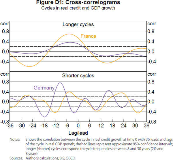
Footnotes
The authors are from the Reserve Bank of Australia's Economic Research Department. All views expressed are those of the authors and in no way represent the views of the Reserve Bank of Australia or its Board. [*]
For example, the Bank for International Settlements' countercyclical capital buffer and the Bank of England's new stress testing framework. [1]
Schüler et al (2017) allows the frequency range to vary by country based on multivariate spectral density results, and so do not assume the length of the financial and business cycles. [2]
Some papers, such as Priestley (1965) and Bayram and Baraniuk (2000), develop methods for estimating the spectral densities of non-stationary processes, referred to as time-varying power spectra. [3]
See Appendix A for data sources and sample periods. Credit covers loans to, and debt securities issued by, the private non-financial sector; this measure will not capture credit provided by other sources, such as shadow banks. [4]
While the credit gap and credit-to-GDP gap have been commonly used to measure the financial cycle, there is little theory behind these measures. In contrast to the output gap, it is not clear what the level of potential credit is or what distortion makes credit deviate from its potential. [5]
We use the variables in level terms for turning point analysis. [6]
For the bootstrapping, we use a Gaussian kernel to smooth the cross-spectra and assume the errors between the smoothed and non-smoothed cross-spectra come from a chi-squared distribution with two degrees of freedom. For more information, see Franke and Härdle (1992) and Berkowitz and Diebold (1998). [7]
The conditions we use are consistent with those used in Harding and Pagan (2002); a cycle needs to be at least five quarters long, a contraction or expansion needs to be at least two quarters long and peaks and troughs need to alternate. [8]
Similar results are found using a Hodrick-Prescott filter, where lambda is chosen to optimise the unfiltered spectral densities between 8 and 30 years, and 2½ and 8 years. These filtering methods suffer from end-point problems, so care needs to be taken when interpreting the beginning and end of the filtered series. [9]
We do not compare the synchronisation of the shorter and longer cycles, since they will have low synchronisation by construction. [10]
However, the presence of two dominant cycles could also be the result of changes in the co-movement in the data over time. [11]
We choose 1980 for two main reasons: a long enough sample is required for stationarity purposes and in order to capture longer cycles; and around this period many countries went through a period of financial liberalisation, so there is likely to be a structural break between the 1970s and the 1980s. However, we acknowledge that structural breaks are likely to have occurred in some of these countries since 1980. [12]
This database covers the period 1870 to 2013. Due to data availability, the time period varies for each country. Note that the only economic variable used in this robustness check is GDP growth, since this database does not provide employment or unemployment data. [13]
The turning point method is typically used on monthly and quarterly data; annual data will only be able to pick up major contractions in the cycles, and therefore the cycles are typically longer (Harding 2002). As such, we do not run this robustness check with annual data using the turning point method. [14]
We would expect the concordance statistic to be 0.5 for two random series since they do not have a unit root (i.e. there is no drift in the series). It takes drift common to both series to increase the expectation of the concordance statistic above 0.5 (McDermott and Scott 2000). [15]
For the cross-correlograms for France and Germany, see Figure D1. [16]
The phase spectrum can only be meaningfully interpreted at frequencies for which spectral mass is high. [17]
This analysis only includes data from 1980 onwards, since we believe that the nature of the relationship between GDP growth and credit growth is likely to have changed during financial liberalisation. [18]
In this paper, we do not discuss changes to prudential regulation and financial system deregulation, which have affected both real and financial variables and may distort the frequencies that we detect in the data. [19]
We will mostly ignore the role of fiscal policy in this paper. [20]
References
Adrian T and HS Shin (2010), ‘Liquidity and Leverage’, Journal of Financial Intermediation, 19(3), pp 418–437.
Agur I and M Demertzis (2015), ‘Will Macroprudential Policy Counteract Monetary Policy's Effects on Financial Stability?’, IMF Working Paper No WP/15/283.
Aikman D, AG Haldane and BD Nelson (2015), ‘Curbing the Credit Cycle’, The Economic Journal, 125(585), pp 1072–1109.
Alpanda S, G Cateau and C Meh (2014), ‘A Policy Model to Analyze Macroprudential Regulations and Monetary Policy’, BIS Working Papers No 461.
Azariadis C, L Kaas and Y Wen (2015), ‘Self-Fulfilling Credit Cycles’, Federal Reserve Bank of St. Louis Working Paper No 2015-005B, rev November.
Bayram M and R Baraniuk (2000), ‘Multiple Window Time-Varying Spectrum Estimation’, in WJ Fitzgerald, RL Smith, AT Walden and P Young (eds), Nonlinear and Nonstationary Signal Processing, Cambridge University Press, Cambridge, pp 292–316.
Berkowitz J and FX Diebold (1998), ‘Bootstrapping Multivariate Spectra’, The Review of Economics and Statistics, 80(4), pp 664–666.
Bernanke BS and M Gertler (1989), ‘Agency Costs, Net Worth, and Business Fluctuations’, The American Economic Review, 79(1), pp 14–31.
Bernanke BS, M Gertler and S Gilchrist (1999), ‘The Financial Accelerator in a Quantitative Business Cycle Framework’, in JB Taylor and M Woodford (eds), Handbook of Macroeconomics: Volume 1C, Handbooks in Economics 15, Elsevier Science, Amsterdam, pp 1341–1393.
Borio C (2012), ‘The Financial Cycle and Macroeconomics: What Have We Learnt?’, BIS Working Papers No 395.
Borio C, C Furfine and P Lowe (2001), ‘Procyclicality of the Financial System and Financial Stability: Issues and Policy Options’, in Marrying the Macro- and Microprudential Dimensions of Financial Stability, BIS Papers No 1, BIS, Basel, pp 1–57.
Borio C and P Lowe (2002), ‘Asset Prices, Financial and Monetary Stability: Exploring the Nexus’, BIS Working Papers No 114.
Borio C and H Zhu (2012), ‘Capital Regulation, Risk-Taking and Monetary Policy: A Missing Link in the Transmission Mechanism?’, Journal of Financial Stability, 8(4), pp 236–251.
Bruno V and HS Shin (2015), ‘Capital Flows and the Risk-Taking Channel of Monetary Policy’, Journal of Monetary Economics, 71, pp 119–132.
Bry G and C Boschan (1971), Cyclical Analysis of Time Series: Selected Procedures and Computer Programs, Technical Paper 20, National Bureau of Economic Research, New York.
Cerutti E, S Claessens and L Laeven (2015), ‘The Use and Effectiveness of Macroprudential Policies: New Evidence’, IMF Working Paper No WP/15/61.
Claessens S, MA Kose and ME Terrones (2011), ‘Financial Cycles: What? How? When?’, IMF Working Paper No WP/11/76.
Cochrane JH (2008), ‘Financial Markets and the Real Economy’, in R Mehra (ed), Handbook of the Equity Risk Premium, Handbooks in Finance, Elsevier, Amsterdam pp 237–325.
Comin D and M Gertler (2006), ‘Medium-Term Business Cycles’, The American Economic Review, 96(3), pp 523–551.
Drehmann M, C Borio and K Tsatsaronis (2012), ‘Characterising the Financial Cycle: Don't Lose Sight of the Medium Term!’, BIS Working Papers No 380.
Dunstan A (2014), ‘The Interaction between Monetary and Macro-Prudential Policy’, Reserve Bank of New Zealand Bulletin, 77(2), pp 15–25.
Fisher I (1933), ‘The Debt-Deflation Theory of Great Depressions’, Econometrica, 1(4), pp 337–357.
Fostel A and J Geanakoplos (2008), ‘Leverage Cycles and the Anxious Economy’, The American Economic Review, 98(4), pp 1211–1244.
Franke J and W Härdle (1992), ‘On Bootstrapping Kernel Spectral Estimates’, The Annals of Statistics, 20(1), pp 121–145.
Galati G, I Hindrayanto, SJ Koopman and M Vlekke (2016), ‘Measuring Financial Cycles with a Model-Based Filter: Empirical Evidence for the United States and the Euro Area’, De Nederlandsche Bank Working Paper No 495.
Gambacorta L (2009), ‘Monetary Policy and the Risk-Taking Channel’, BIS Quarterly Review, December, pp 43–53.
Geanakoplos J (2010), ‘The Leverage Cycle’, in D Acemoglu, K Rogoff and M Woodford (eds), NBER Macroeconomics Annual 2009, Vol 24, University of Chicago Press, Chicago, pp 1–65.
Gertler M and P Karadi (2011), ‘A Model of Unconventional Monetary Policy’, Journal of Monetary Economics, 58(1), pp 17–34.
Gertler M and N Kiyotaki (2011), ‘Financial Intermediation and Credit Policy in Business Cycle Analysis’, in BM Friedman and M Woodford (eds), Handbook of Monetary Economics: Volume 3A, Handbooks in Economics, Elsevier, Amsterdam, pp 547–599.
Guibourg G, M Jonsson, B Lagerwall and C Nilsson (2015), ‘Macroprudential Policy – Effects on the Economy and the Interaction with Monetary Policy’, Sveriges Riksbank Economic Review, 2015(2), pp 29–46.
Gurley JG and ES Shaw (1955), ‘Financial Aspects of Economic Development’, The American Economic Review, 45(4), pp 515–538.
Hamilton JD (2017), ‘Why You Should Never Use the Hodrick-Prescott Filter’, Unpublished manuscript, University of California, San Diego, 9 January.
Harding D (2002), ‘The Australian Business Cycle: A New View’, Paper presented at the Melbourne Institute and The Australian Economic and Social Outlook Conference 2002 ‘Towards Opportunity and Prosperity’, Melbourne, 4–5 April.
Harding D and A Pagan (2002), ‘Dissecting the Cycle: A Methodological Investigation’, Journal of Monetary Economics, 49(2), pp 365–381.
Harding D and A Pagan (2006), ‘Synchronization of Cycles’, Journal of Econometrics, 132(1), pp 59–79.
Harimohan R and B Nelson (2014), ‘How Might Macroprudential Capital Policy Affect Credit Conditions?’, Bank of England Quarterly Bulletin, 54(3) Q3, pp 287–303.
Jordà Ò, M Schularick and AM Taylor (2015), ‘Leveraged Bubbles’, Journal of Monetary Economics, 76(Supplement), pp S1–S20.
Jordà Ò, M Schularick and AM Taylor (2017), ‘Macrofinancial History and the New Business Cycle Facts’, in M Eichenbaum and JA Parker (eds), NBER Macroeconomics Annual 2016, Vol 31, University of Chicago Press, Chicago, pp 213–263.
Juselius M, C Borio, P Disyatat and M Drehmann (2017), ‘Monetary Policy, the Financial Cycle, and Ultra-Low Interest Rates’, International Journal of Central Banking, 13(3), pp 55–89.
Kindleberger CP (1978), Manias, Panics, and Crashes: A History of Financial Crises, Basic Books, New York.
Kiyotaki N and J Moore (1997), ‘Credit Cycles’, Journal of Political Economy, 105(2), pp 211–248.
Lowe P (1992), ‘The Impact of Financial Intermediaries on Resource Allocation and Economic Growth’, RBA Research Discussion Paper No 9213.
Maddaloni A and J-L Peydró (2013), ‘Monetary Policy, Macroprudential Policy, and Banking Stability: Evidence from the Euro Area’, International Journal of Central Banking, 9(1), pp 121–169.
McDermott CJ and A Scott (2000), ‘Concordance in Business Cycles’, IMF Working Paper No WP/00/37.
Minsky HP (1977), ‘A Theory of Systemic Fragility’, in EI Altman and AW Sametz (eds), Financial Crises: Institutions and Markets in A Fragile Environment, John Wiley and Sons, New York, pp 138–152.
Modigliani F and MH Miller (1958), ‘The Cost of Capital, Corporation Finance and the Theory of Investment’, The American Economic Review, 48(3), pp 261–297.
Phillips PCB and S Jin (2015), ‘Business Cycles, Trend Elimination, and the HP Filter’, Cowles Foundation Discussion Paper No 2005.
Praet P (2016), ‘Financial Cycles and Monetary Policy’, Panel discussion on ‘International Monetary Policy’ at ‘Business Cycles, Financial Markets, and Monetary Policy with Special Applications to China’, A conference sponsored by the European Central Bank, Tsinghua University, Federal Reserve Bank of San Francisco, Shanghai Advanced Institution of Finance (SAIF), Northwestern University and Federal Reserve Bank of Atlanta, Beijing, 30 August–1 September.
Priestley MB (1965), ‘Evolutionary Spectra and Non-Stationary Processes’, Journal of the Royal Statistical Society Series B (Methodological), 27(2), pp 204–229.
Rajan RG (2005), ‘Has Financial Development Made the World Riskier?’, NBER Working Paper No 11728.
Reinhart CM and KS Rogoff (2009), This Time is Different: Eight Centuries of Financial Folly, Princeton University Press, Princeton.
Rünstler G and M Vlekke (2016), ‘Business, Housing and Credit Cycles’, European Central Bank Working Paper Series No 1915.
Sargent TJ and N Wallace (1981), ‘Some Unpleasant Monetarist Arithmetic’, Federal Reserve Bank of Minneapolis Quarterly Review, 5(3), pp 1–17.
Schenk-Hoppé KR (2001), ‘Economic Growth and Business Cycles: A Critical Comment on Detrending Time Series’, Studies in Nonlinear Dynamics and Econometrics, 5(1), Article 6.
Schularick M and AM Taylor (2012), ‘Credit Booms Gone Bust: Monetary Policy, Leverage Cycles, and Financial Crises, 1870–2008’, The American Economic Review, 102(2), pp 1029–1061.
Schüler YS, PP Hiebert and TA Peltonen (2017), ‘Coherent Financial Cycles for G-7 Countries: Why Extending Credit Can Be an Asset’, European Systemic Risk Board Working Paper Series No 43.
Sengupta R (2010), ‘Alt-A: The Forgotten Segment of the Mortgage Market’, Federal Reserve Bank of St. Louis Review, 92(1), pp 55–71.
Smets F (2013), ‘Financial Stability and Monetary Policy: How Closely Interlinked?’, Sveriges Riksbank Economic Review, 2012(3), pp 121–160.
Stein JC (2013), ‘Overheating in Credit Markets: Origins, Measurement, and Policy Responses’, Breakfast Keynote Address given at Federal Reserve Bank of St. Louis and Center for Social Development Research Symposium ‘Restoring Household Financial Stability after the Great Recession: Why Household Balance Sheets Matter’, St. Louis, 5–7 February.
Strohsal T, CR Proaño and J Wolters (2015), Characterizing the Financial Cycle: Evidence from a Frequency Domain Analysis, Bundesbank Discussion Paper No 22/2015, Deutsche Bundesbank, Frankfurt am Main.
Svensson LEO (2016), ‘Cost-Benefit Analysis of Leaning against the Wind: Are Costs Larger Also with Less Effective Macroprudential Policy?’, IMF Working Paper No WP/16/3.
Tinbergen J (1952), On the Theory of Economic Policy, Contributions to Economic Analysis No 1, North Holland Publishing Company, Amsterdam.