RDP 1977-06: Interest Rates and Exchange Rate Expectations in the RBA76 Model 3. Measuring and Modelling the Debenture Rate
October 1977
3.1 Measurement
A major problem in an investigation of this type is the choice of data to proxy a representative market-determined interest rate. For the current project the rate chosen is a weighted (by value of sales on the Melbourne Stock Exchange) average redemption yield of ‘long-terra’ (defined here as eight years or longer) debentures of major companies.[4] This choice is made so that the private financial assets whose rates of return are represented in the model are reasonably comparable with the bond rate as defined in this study. There remains room, however, for further experiments with alternative measures of private sector interest rates.
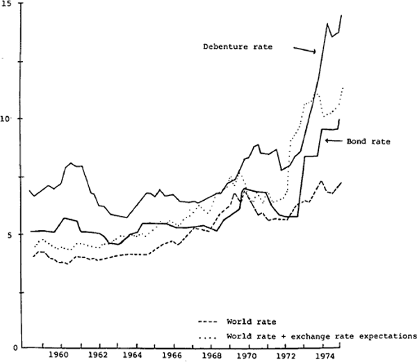
Figure 1 presents the debenture rate as measured in this study together with the redemption yield on Commonwealth government securities with ten years to maturity. Also shown are the measure of the rest-of-world interest rates used in the RBA76 model and this measure adjusted for the expected rate of exchange rate change; the derivation of the exchange rate expectations adjustment is discussed in Section 5 of this paper.

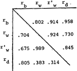
The graph, together with Table 1, indicates a high degree of correlation between the debenture and bond rates, and a somewhat weaker relationship between each of these and the world interest rate adjusted for exchange rate expectations.
| 1959 to 1975 |
 |
|---|---|
|
rb bond rate, rd debenture rate, rw world
rate, ($US) |
|
In the period to 1970 the debenture rate appears to incorporate a fairly constant risk premium over the bond rate, with major turning points in the bond rate generally preceding those of the debenture rate series. The relationship between the two rates is, however, much less clear in the later years. It is notable that the upward path of the debenture rate over the 1970–74 period was considerably smoother than that of the bond rate, which could suggest an episodic response of bond rates to increasing market rates.
In the short run there is at times quite divergent behaviour of the world rate and the domestic rates. Thus in 1970 to 1972 the world rate was relatively low at a time when the two domestic rates were relatively high. Then the world rate, adjusted for exchange rate expectations, rose sharply, in advance of the rise in domestic rates. At the end of the period, the fall and later rise in the world rate preceded a similar movement in the debenture rate.
3.2 Modelling the debenture rate
The specification of the debenture rate equation in the model is similar to that for other endogenous variables, in that the debenture rate is assumed to adjust, with a lag, to an equilibrium level, with the speed of adjustment also dependent on other variables. This procedure is based on the theory of non-tatonnement processes, where prices (e.g. the debenture rate) are set by reference to prices in related markets, with adjustment influenced by various measures of quantity disequilibrium.[5]
In Models A, B and C, in which the bond rate adjusts to a target rate determined by the monetary growth rate, the debenture rate (rd) is assumed to adjust to a weighted average of the bond rate (rb) and the world rate adjusted for the influence of exchange rate expectations (rw+ ξ). These two financial sector interest rates are in the demand functions for money and bonds, and in the desired net foreign demand for Australian assets in the model as the bond rate and interest rates in the rest of the world are assumed to represent the rates of return most relevant for participants in the debenture market. The use of this basic adjustment term permits a simple test of the relative importance of interest rates in the rest of the world and in the market for Commonwealth government securities in the determination of the debenture rate.
In Model D, in which the causation between the debenture rate and the bond rate is reversed, the target bond rate is defined as the debenture rate and the debenture rate is assumed to adjust to the world rate adjusted for exchange rate expectations. The alternative specifications represent two important ways to model the interactions suggested by figure 1. The model estimates for the full period represent the average behaviour over the sample period, and so cannot allow for a changing relationship which might be suggested by figure 1. However, the estimation results are capable of indicating which model best fits the average experience over the past sixteen years.
There have been two measures of quantity disequilibrium considered likely to influence the
adjustment of the debenture rate toward the equilibrium level. The first is the gap between
desired investment ( , defined
to be consistent with that in the investment equation in the model) and a proxy for retained
earnings of companies, a constant proportion of net-of-tax “company
profits”. “Company Profits” is defined simply as nominal income (Py) less
wage payments (WL); this is a very crude proxy for company profits, and the term is entered
with an independent parameter to avoid biassing the results with an inappropriate
restriction.
A second measure of market disequilibrium, the excess stock demand for money (log  − log
M/p) was included in the equation in some experiments in order to test
whether monetary disequilibrium has any direct effect on rates of return in private sector
asset markets.
The first of the two quantity disequilibrium terms referred to above is significant and numerically important in all models, while the second has a somewhat unstable influence. In particular, the performance of monetary disequilibrium depends on the precise specification of the policy reaction function for the bond rate, and because of this it is omitted from the models presented in this paper. It is perhaps worth reporting that whenever monetary disequilibrium is significant in the equation for the debenture rate it has a negative sign, indicating that in the short run the price expectations effect dominates the liquidity effect which would be suggested by a positive sign.[6]
The company debenture rate equation in the model is written in its most general form as follows:[7]
As noted in the introduction, there are four models considered in this paper. Because of the way in which the whole model is estimated simultaneously, the parameters of the equation for the company debenture rate are different in each model. Table 2 sets out the four different sets of estimates.[8] They are sufficiently similar that a general discussion can be provided here, to be supplemented below.
Several aspects of these results are interesting. In Models A and B, the estimated weight on the bond rate in defining the equilibrium debenture rate is high, which appears to support the usual approach to the determination of interest rates; the results of Model C, however, assign a greater relative importance to the influence of the world interest rate, although in this case β3, is still in the region of 5. In each of the models the excess demand for investment funds significantly influences the adjustment of the debenture rate, and further evidence is required before a firm judgement can be reached as to the extent of short-run control the monetary authorities are able to exercise over interest rates in the private sector.
The parameters of the equation for the debenture rate of Model D, which tests an alternative model of policy reaction, are similar to their counterparts in Models A, B and C (except that β3, is constrained to unity), and the fit statistics of the bond rate and debenture rate equations in each model are comparable.[9] The question of the direction of causation between bond rates and debenture rates remains unclear from the estimation evidence.
| Model A | Model B | Model C | Model D | |
|---|---|---|---|---|
| α1 | 0.28 (5.67) |
0.41 (5.17) |
0.38 (4.65) |
0.29 (6.65) |
| β1 | 0.8 (4.72) |
0.8 (5.52) |
1.0 (6.25) |
0.6 (4.32) |
| β2 | 0.006 (3.28) |
0.005 (3.00) |
0.005 (3.16) |
0.004 (3.23) |
| β3 | 0.25 (.72) |
0.10 (.48) |
0.48 (2.18) |
1.0 (constrained) |
Footnotes
The data are discussed in the appendix. [4]
Some economists would prefer to define supply and demand functions for debentures and use these to define a debenture rate which clears the market, although this is not necessarily appropriate if markets are not continuously clearing. [5]
The specification does not allow for a distributed lag in which it would be possible for the liquidity effect to operate initially, with the expectations effect dominating in the longer run. [6]
All variables are defined as in the basic RBA76 model. Apart from those defined in the text, t represents the average company tax rate and MPK the marginal product of capital. [7]
The figures in brackets are t-ratios calculated from the parameter estimates and their asymptotic standard errors. [8]
The estimates of parameters and fit statistics for all equations in the models of this paper are available on request. They are similar to the corresponding parameters in the basic model set [9]
