RDP 8701: The Australian Demand Function for Money: Another Look at Stability 5. Stability in the 1980s: Results of Further Tests
January 1987
- Download the Paper 958KB
In the First half of the 1980s, the Australian financial system has undergone substantial, and rapid, deregulation. Amongst the important changes have been:
- the lifting of restrictions on interest rates paid on most bank deposits in December 1980;
- the introduction of tender arrangements for marketing long-term government debt in August 1982;
- floating of the Australian dollar and the abolition of most exchange controls in December 1983;
- lifting of restrictions on terms and maturities on bank deposits in August 1984;
- the licensing of a number of new banks, from early 1985.
These events have had a profound influence on the financial system, and particularly on the monetary aggregates. The freeing-up of the banking system improved the banks' competitive position vis-a-vis non-bank financial intermediaries, and led to a shift of business between the two sectors. To the extent that the financial system generally became more competitive and efficient, there could also have been some shift from direct financing to intermediation.[7] Both of these factors could affect the relationship between observed levels of the money stock, interest rates and real activity. In addition, the floating of the exchange rate might be expected to affect the variability of domestic interest rates, and the nature of the money supply process. In a simple analytical framework assuming a fixed exchange rate and perfect capital markets, the quantity of money supplied is seen as adjusting to the quantity demanded. Under a floating regime, this is no longer so (in the absence of systematic central bank intervention). This may have implications for the estimated relationship between the money stock and other variables.
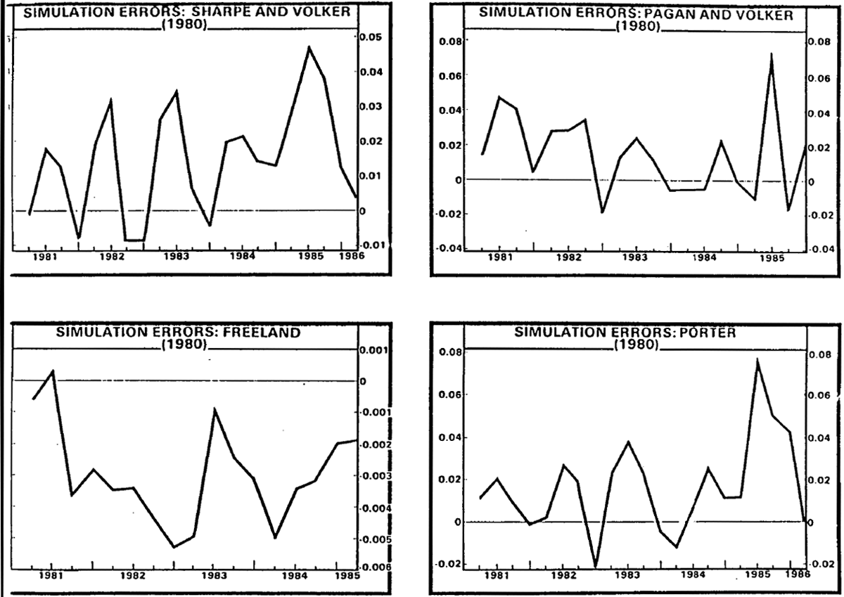
For these reasons, an additional test is performed on equations SV-3, PO-3, FR-3 and PV-3, namely the post-sample predictive test developed by Davidson et. al. (1978). This consists of estimating the model up to some date T, which we have taken to be December 1980, and then using the model for (static) simulation past T (up to around the end of 1985 in this case). Davidson et. al. (1978) develop a formal test statistic for the forecast residuals, which is easy to compute.
Figure 5 shows plots of the simulation errors. The absolute size of the errors is large in several cases. The scale on the graph is calibrated in logs, so that the figures indicate proportionate errors – with peaks between 5 and 8 per cent. It is notable that a large error in mid 1985, the period immediately following the abandoning of the conditional projection for M3 (in January 1985), shows up clearly in all three equations in which the test is conducted that far out.
So much for the absolute errors. Table 7 gives the formal test statistics, based on the sums of squared residuals.
| Equation no: | Test * Statistic |
Critical Value | |
|---|---|---|---|
| 1% | 5% | ||
| SV-3 | 53.4 | 38.9 | 32.7 |
| PO-3 | 44.3 | 38.9 | 32.7 |
| FR-3 | 103.8 | 33.4 | 27.6 |
| PV-3 | 56.2 | 37.6 | 31.4 |
* In a model of the form yt = xt ′β + εt, εt
~ (0, σ2), estimated using T observations, and simulated using
actual values for the xt for periods t = T+1, … T+2, under the
null hypothesis of no change in the β (and assuming σ
2 is unchanged) the test statistic is where  is the estimate of the variance of the error
within the sample is the estimate of the variance of the error
within the sample . .
|
|||
All of the test statistics reported here convincingly reject the null hypothesis of stability.

Of course, this test is likely to be affected by the heteroskedasticity problem, just as were the tests in Section 4. If the variance is growing over time, it seems, intuitively at least, that the Davidson et. al. test would be biased against the null hypothesis. Even so, it seems likely that this problem would have to be severe in order to completely invalidate the conclusions, especially as they are consistent with the earlier results.
It might be argued that a five-year simulation period is an unreasonably long period over which to test a model. But allowing estimation up to June 1984, and simulating over only 7 quarters does not substantially change the results.
Footnote
These points are brought out more fully in a Research Report “Changing Patterns of Finance”, published in the Reserve Bank Bulletin, May 1985. [7]